
ProUCL Version 5.1
User Guide
Statistical Software for Environmental Applications
for Data Sets with and without Nondetect
Observations
R E S E A R C H A N D D E V E L O P M E N T

2

Notice: Although this work was reviewed by EPA and approved for publication, it may not necessarily reflect official
Agency policy. Mention of trade names and commercial products does not constitute endorsement or
recommendation for use.
129cmb07
ProUCL Version 5.1
User Guide
Statistical Software for Environmental Applications
for Data Sets with and without Nondetect
Observations
Prepared for:
Felicia Barnett, Director
ORD Site Characterization and Monitoring Technical Support Center (SCMTSC)
Superfund and Technology Liaison, Region 4
U.S. Environmental Protection Agency
61 Forsyth Street SW, Atlanta, GA 30303
Prepared by:
Anita Singh, Ph.D.
and Robert Maichle
Lockheed Martin/SERAS
IS&GS-CIVIL
2890 Woodbridge Ave
Edison NJ 08837
EPA/600/R-07/041
October 2015
www.epa.gov
U.S. Environmental Protection Agency
Office of Research and Development
Washington, DC 20460
1
NOTICE
The United States Environmental Protection Agency (U.S. EPA) through its Office of Research and
Development (ORD) funded and managed the research described in ProUCL Technical Guide and
methods incorporated in the ProUCL software. It has been peer reviewed by the U.S. EPA and approved
for publication. Mention of trade names or commercial products does not constitute endorsement or
recommendation by the U.S. EPA for use.
All versions of the ProUCL software including the current version ProUCL 5.1 have been
developed by Lockheed Martin, IS&GS - CIVIL under the Science, Engineering, Response and
Analytical contract with the U.S. EPA and is made available through the U.S. EPA Technical
Support Center (TSC) in Atlanta, Georgia (GA).
Use of any portion of ProUCL that does not comply with the ProUCL Technical Guide is not
recommended.
ProUCL contains embedded licensed software. Any modification of the ProUCL source code
may violate the embedded licensed software agreements and is expressly forbidden.
ProUCL software provided by the U.S. EPA was scanned with McAfee VirusScan version 4.5.1
SP1 and is certified free of viruses.
With respect to ProUCL distributed software and documentation, neither the U.S. EPA nor any of their
employees, assumes any legal liability or responsibility for the accuracy, completeness, or usefulness of
any information, apparatus, product, or process disclosed. Furthermore, software and documentation are
supplied “as-is” without guarantee or warranty, expressed or implied, including without limitation, any
warranty of merchantability or fitness for a specific purpose.
ProUCL software is a statistical software package providing statistical methods described in various U.S.
EPA guidance documents. ProUCL does not describe U.S. EPA policies and should not be considered to
represent U.S. EPA policies.

2
Minimum Hardware Requirements
ProUCL 5.1 will function but will run slowly and page a lot.
Intel Pentium 1.0 gigahertz (GHz)
45 MB of hard drive space
512 MB of memory (RAM)
CD-ROM drive or internet connection
Windows XP (with SP3), Vista (with SP1 or later), and Windows 7.
ProUCL 5.1 will function but some titles and some Graphical User Interfaces (GUIs) will need to be
scrolled. Definition without color will be marginal.
800 by 600 Pixels
Basic Color is preferred
Preferred Hardware Requirements
1 GHz or faster Processor.
1 gigabyte (GB) of memory (RAM)
1024 by 768 Pixels or greater color display
Software Requirements
ProUCL 5.1 has been developed in the Microsoft .NET Framework 4.0 using the C# programming
language. To properly run ProUCL 5.1 software, the computer using the program must have the .NET
Framework 4.0 pre-installed. The downloadable .NET Framework 4.0 files can be obtained from one of
the following websites:
http://msdn.microsoft.com/netframework/downloads/updates/default.aspx
http://www.microsoft.com/en-us/download/details.aspx?id=17851
Quicker site for 32 Bit Operating systems
http://www.microsoft.com/en-us/download/details.aspx?id=24872
Use this site if you have a 64 Bit operating system
3
Installation Instructions when Downloading ProUCL 5.1 from the EPA Web Site
Download the file SETUP.EXE from the EPA Web site and save to a temporary location.
Run the SETUP.EXE program. This will create a ProUCL directory and two folders:
1) The USER GUIDE (this document), and 2) DATA (example data sets).
To run the program, use Windows Explorer to locate the ProUCL application file, and
Double click on it, or use the RUN command from the start menu to locate the
ProUCL.exe file, and run ProUCL.exe.
To uninstall the program, use Windows Explorer to locate and delete the ProUCL folder.
Caution: If you have previous versions of the ProUCL, which were installed on your computer, you
should remove or rename the directory in which earlier ProUCL versions are currently located.
Installation Instructions when Copying ProUCL 5.1 from a CD
Create a folder named ProUCL 5.1 on a local hard drive of the machine you wish to
install ProUCL 5.1.
Extract the zipped file ProUCL.zip to the folder you have just created.
Run ProUCL.exe.
Note: If you have extension turned off, the program will show with the name ProUCL in your directory
and have an Icon with the label ProUCL.
Creating a Shortcut for ProUCL 5.1 on Desktop
To create a shortcut of the ProUCL program on your desktop, go to your ProUCL
directory and right click on the executable program and send it to desktop. A ProUCL
icon will be displayed on your desktop. This shortcut will point to the ProUCL directory
consisting of all files required to execute ProUCL 5.1.
Caution: Because all files in your ProUCL directory are needed to execute the ProUCL software, one
needs to generate a shortcut using the process described above. Simply dragging the ProUCL executable
file from Window Explorer onto your desktop will not work successfully (an error message will appear)
as all files needed to run the software are not available on your desktop. Your shortcut should point to the
directory path with all required ProUCL files.

4
ProUCL 5.1
Software ProUCL version 5.1 (ProUCL 5.1), its earlier versions: ProUCL version 3.00.01, 4.00.02,
4.00.04, 4.00.05, 4.1.00, 4.1.01, and ProUCL 5.0.00, associated Facts Sheet, User Guides and Technical
Guides (e.g., EPA 2010a, 2010b, 2013a, 2013b) can be downloaded from the following EPA website:
http://www.epa.gov/osp/hstl/tsc/software.htm
http://www.epa.gov/osp/hstl/tsc/softwaredocs.htm
Material for ProUCL webinars offered in March 2011, and relevant literature used in the development of
various ProUCL versions can also be downloaded from the above EPA website.
Contact Information for all Versions of ProUCL
Since 1999, the ProUCL software has been developed under the direction of the Technical Support Center
(TSC). As of November 2007, the direction of the TSC is transferred from Brian Schumacher to Felicia
Barnett. Therefore, any comments or questions concerning all versions of ProUCL software should be
addressed to:
Felicia Barnett, Director
ORD Site Characterization and Monitoring Technical Support Center (SCMTSC)
Superfund and Technology Liaison, Region 4
U.S. Environmental Protection Agency
61 Forsyth Street SW, Atlanta, GA 30303-8960
barnett.felicia@epa.gov
(404)562-8659
Fax: (404) 562-8439
5
Getting Started
The look and feel of ProUCL 5.1 is similar to that of ProUCL 5.0; and they share the same names for
modules and drop-down menus. The functionality and the use of the methods and options available in
ProUCL 5.1 have been illustrated using Screen shots of output screens generated by ProUCL 5.1.
ProUCL 5.1 uses a pull-down menu structure, similar to a typical Windows program. For modules where
no changes have been made in ProUCL since 2010 (e.g., Sample Sizes), screen shots as used in ProUCL
5.0 documents have been used in ProUCL 5.1 documents. Some of the screen shots generated using
ProUCL 5.1 might have ProUCL 5.0 in their titles as those screen shots have not been re-generated and
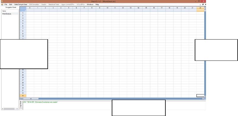
replaced. The screen shown below appears when the program is executed.
The above screen consists of three main window panels:
The MAIN WINDOW displays data sheets and outputs results from the procedure used.
The NAVIGATION PANEL displays the name of data sets and all generated outputs.
o The navigation panel can hold up to 40 output files. In order to see more files (data
files or generated output files), one can click on Widow Option.
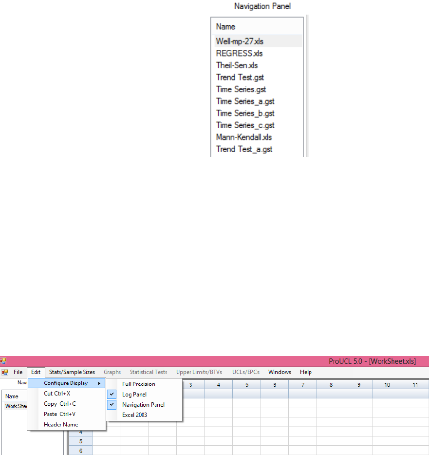
o In the NAVIGATION PANEL, ProUCL assigns self explanatory names to output
files generated using the various modules of ProUCL. If the same module (e.g.,
Time Series Plot) is used many times, ProUCL identifies them by using letters a, b,
c,...and so on as shown below.
← Main
Window
Navigation
Panel
↓
← Log Panel
6
o The user may want to assign names of his choice to these output files when saving
them using the "Save" or "Save As" Options.
The LOG PANEL displays transactions in green, warning messages in orange, and errors in
red. For an example, when one attempts to run a procedure meant for left-censored data sets
on a full-uncensored data set, ProUCL 5.1 will output a warning in orange in this panel.
o Should both panels be unnecessary, you can choose Configure ► Panel ON/OFF.
The use of this option gives extra space to see and print out the statistics of interest. For example, one
may want to turn off these panels when multiple variables (e.g., multiple quantile-quantile [Q-Q] plots)
are analyzed and goodness-of-fit (GOF) statistics and other statistics may need to be captured for all of
the selected variables. The following screen was generated using ProUCL 5.0. An identical screen will be
generated using ProUCL 5.1 with title name as ProUCL 5.1 - [WorkSheet.xls].
7
EXECUTIVE SUMMARY
The main objective of the ProUCL software funded by the United States Environmental Protection
Agency (EPA) is to compute rigorous statistics to help decision makers and project teams in making good
decisions at a polluted site which are cost-effective, and protective of human health and the environment.
The ProUCL software is based upon the philosophy that rigorous statistical methods can be used to
compute reliable estimates of population parameters and decision making statistics including: the upper
confidence limit (UCL) of the mean, the upper tolerance limit (UTL), and the upper prediction limit
(UPL) to help decision makers and project teams in making correct decisions. A few commonly used text
book type methods (e.g., Central Limit Theorem [CLT], Student's t-UCL) alone cannot address all
scenarios and situations occurring in environmental studies. Since many environmental decisions are
based upon a 95 percent (%) UCL (UCL95) of the population mean, it is important to compute UCLs of
practical merit. The use and applicability of a statistical method (e.g., student's t-UCL, CLT-UCL,
adjusted gamma-UCL, Chebyshev UCL, bootstrap-t UCL) depend upon data size, data skewness, and
data distribution. ProUCL computes decision statistics using several parametric and nonparametric
methods covering a wide-range of data variability, distribution, skewness, and sample size. It is
anticipated that the availability of the statistical methods in the ProUCL software covering a wide range
of environmental data sets will help the decision makers in making more informative and correct
decisions at Superfund and Resource Conservation and Recovery Act (RCRA) sites.
It is noted that for moderately skewed to highly skewed environmental data sets, UCLs based on the CLT
and the Student's t-statistic fail to provide the desired coverage (e.g., 0.95) to the population mean even
when the sample sizes are as large as 100 or more. The sample size requirements associated with the CLT
increases with skewness. It would be incorrect to state that a CLT or Student's statistic based UCLs are
adequate to estimate Exposure Point Concentrations (EPC) terms based upon skewed data sets. These
facts have been described in the published documents (Singh, Singh, and Engelhardt [1997, 1999]; Singh,
Singh, and Iaci 2002; Singh and Singh 2003; and Singh et al. 2006) summarizing simulation experiments
conducted on positively skewed data sets to evaluate the performances of the various UCL computation
methods. The use of a parametric lognormal distribution on a lognormally distributed data set yields
unstable impractically large UCLs values, especially when the standard deviation (sd) of the log-
transformed data becomes greater than 1.0 and the data set is of small size less than (<) 30-50. Many
environmental data sets can be modeled by a gamma as well as a lognormal distribution. The use of a
gamma distribution on gamma distributed data sets tends to yield UCL values of practical merit.
Therefore, the use of gamma distribution based decision statistics such as UCLs, UPLs, and UTLs should
not be dismissed by stating that it is easier to use a lognormal model to compute these upper limits.
The suggestions made in ProUCL are based upon the extensive experience of the developers in
environmental statistical methods, published environmental literature, and procedures described in many
EPA guidance documents. These suggestions are made to help the users in selecting the most appropriate
UCL to estimate the EPC term which is routinely used in exposure assessment and risk management
studies of the USEPA. The suggestions are based upon the findings of many simulation studies described
in Singh, Singh, and Engelhardt (1997, 1999); Singh, Singh, and Iaci (2002); Singh and Singh (2003); and
Singh et al. (2006). It should be pointed out that a typical simulation study does not (cannot) cover all
real world data sets of various sizes and skewness from all distributions. When deemed necessary, the
user may want to consult a statistician to select an appropriate upper limit to estimate the EPC term and
other environmental parameters of interest. For an analyte (data set) with skewness (sd of logged data)
near the end points of the skewness intervals presented in decision tables of Chapter 2 (e.g., Tables 2-9
8
through 2-11), the user may select the most appropriate UCL based upon the site conceptual site model
(CSM), expert site knowledge, toxicity of the analyte, and exposure risks associated with that analyte.
The inclusion of outliers in the computation of the various decision statistics tends to yield inflated values
of those decision statistics, which can lead to poor decisions. Often statistics that are computed for a data
set which includes a few outliers tend to be inflated and represent those outliers rather than representing
the main dominant population of interest (e.g., reference area). Identification of outliers, observations
coming from population(s) other than the main dominant population is suggested, before computing the
decision statistics needed to address project objectives. The project team may want to perform the
statistical evaluations twice, once with outliers and once without outliers. This exercise will help the
project team in computing reliable and defensible decision statistics which are needed to make cleanup
and remediation decisions at polluted sites.
The initial development during 1999-2000 and all subsequent upgrades and enhancements of the ProUCL
software have been funded by U.S. EPA through its Office of Research and Development (ORD).
Initially ProUCL was developed as a research tool for U.S. EPA scientists and researchers of the
Technical Support Center (TSC) and ORD- National Exposure Research Laboratory (NERL), Las Vegas.
Background evaluations, groundwater (GW) monitoring, exposure and risk management and cleanup
decisions in support of the Comprehensive Environmental Recovery, Compensation, and Liability Act
(CERCLA) and RCRA site projects of the U.S. EPA are often derived based upon test statistics such as
the Shapiro-Wilk (S-W) test, t-test, Wilcoxon-Mann-Whitney (WMW) test, analysis of variance
(ANOVA), and Mann-Kendall (MK) test and decision statistics including UCLs of the mean, UPLs, and
UTLs. To address the statistical needs of the environmental projects of the USEPA, over the years
ProUCL software has been upgraded and enhanced to include many graphical tools and statistical
methods described in many EPA guidance documents including: EPA 1989a, 1989b, 1991, 1992a, 1992b,
2000 Multi-Agency Radiation Survey and Site Investigation Manual (MARSSIM), 2002a, 2002b, 2002c,
2006a, 2006b, and 2009. Several statistically rigorous methods (e.g., for data sets with nondetects [NDs])
not easily available in the existing guidance documents and in the environmental literature are also
available in ProUCL 5.0/ProUCL 5.1.
ProUCL 5.1/ProUCL 5.0 has graphical, estimation, and hypotheses testing methods for uncensored-full
data sets and for left-censored data sets including ND observations with multiple detection limits (DLs) or
reporting limits (RLs). In addition to computing general statistics, ProUCL 5.1 has goodness-of-fit (GOF)
tests for normal, lognormal and gamma distributions, and parametric and nonparametric methods
including bootstrap methods for skewed data sets for computation of decision making statistics such as
UCLs of the mean (EPA 2002a), percentiles, UPLs for a pre-specified number of future observations
(e.g., k with k=1, 2, 3,...), UPLs for mean of future k (≥1) observations, and UTLs (e.g., EPA 1992b,
2002b, and 2009). Many positively skewed environmental data sets can be modeled by a lognormal as
well as a gamma model. It is well-known that for moderately skewed to highly skewed data sets, the use
of a lognormal distribution tends to yield inflated and unrealistically large values of the decision statistics
especially when the sample size is small (e.g., <20-30). For gamma distributed skewed uncensored and
left-censored data sets, ProUCL software computes decision statistics including UCLs, percentiles, UPLs
for future k (≥1) observations, UTLs, and upper simultaneous limits (USLs).
For data sets with NDs, ProUCL has several estimation methods including the Kaplan-Meier (KM)
method, regression on order statistics (ROS) methods and substitution methods (e.g., replacing NDs by
DL, DL/2). ProUCL 5.1 can be used to compute upper limits which adjust for data skewness;
specifically, for skewed data sets, ProUCL computes upper limits using KM estimates in gamma
(lognormal) UCL and UTL equations provided the detected observations in the left-censored data set
follow a gamma (lognormal) distribution. Some poor performing commonly used and cited methods such
9
as the DL/2 substitution method and H-statistic based UCL computation method have been retained in
ProUCL 5.1 for historical reasons, and research and comparison purposes.
The Sample Sizes module of ProUCL can be used to develop data quality objectives (DQOs) based
sampling designs and to perform power evaluations needed to address statistical issues associated with a
variety of site projects. ProUCL provides user-friendly options to enter the desired values for the decision
parameters such as Type I and Type II error rates, and other DQOs used to determine the minimum
sample sizes needed to address project objectives. The Sample Sizes module can compute DQO-based
minimum sample sizes needed: to estimate the population mean; to perform single and two-sample
hypotheses testing approaches; and in acceptance sampling to accept or reject a batch of discrete items
such as a lot of drums containing hazardous waste. Both parametric (e.g., t-test) and nonparametric (e.g.,
Sign test, WMW test, test for proportions) sample size determination methods are available in ProUCL.
ProUCL has exploratory graphical methods for both uncensored data sets and for left-censored data sets
consisting of ND observations. Graphical methods in ProUCL include histograms, multiple quantile-
quantile (Q-Q) plots, and side-by-side box plots. The use of graphical displays provides additional insight
about the information contained in a data set that may not otherwise be revealed by the use of estimates
(e.g., 95% upper limits) and test statistics (e.g., two-sample t-test, WMW test). In addition to providing
information about the data distributions (e.g., normal or gamma), Q-Q plots are also useful in identifying
outliers and the presence of mixture populations (e.g., data from several populations) potentially present
in a data set. Side-by-side box plots and multiple Q-Q plots are useful to visually compare two or more
data sets, such as: site-versus-background concentrations, surface-versus-subsurface concentrations, and
constituent concentrations of several GW monitoring wells (MWs). ProUCL also has a couple of classical
outlier test procedures, such as the Dixon test and the Rosner test which can be used on uncensored data
sets as well as on left-censored data sets containing ND observations.
ProUCL has parametric and nonparametric single-sample and two-sample hypotheses testing approaches
for uncensored as well as left-censored data sets. Single-sample hypotheses tests: Student’s t-test, Sign
test, Wilcoxon Signed Rank test, and the Proportion test are used to compare site mean/median
concentrations (or some other threshold such as an upper percentile) with some average cleanup standard,
C
s
(or a not-to-exceed compliance limit, A
0
) to verify the attainment of cleanup levels (EPA, 1989a; 2000,
2006a) at remediated site areas of concern. Single-sample tests such as the Sign test and Proportion test,
and upper limits including UTLs and UPLs are also used to perform intra-well comparisons. Several two-
sample hypotheses tests as described in EPA guidance documents (e.g., 2002b, 2006b, 2009) are also
available in the ProUCL software. The two-sample hypotheses testing approaches in ProUCL include:
Student’s t-test, WMW test, Gehan test and Tarone-Ware (T-W) test. The two-sample tests are used to
compare concentrations of two populations such as site versus background, surface versus subsurface
soils, and upgradient versus downgradient wells.
The Oneway ANOVA module in ProUCL has both classical and nonparametric Kruskal-Wallis (K-W)
tests. Oneway ANOVA is used to compare means (or medians) of multiple groups such as comparing
mean concentrations of areas of concern and to perform inter-well comparisons. In GW monitoring
applications, the ordinary least squares (OLS) regression model, trend tests, and time series plots are used
to identify upwards or downwards trends potentially present in constituent concentrations identified in
wells over a certain period of time. The Trend Analysis module performs the M-K trend test and Theil-
Sen (T-S) trend test on data sets with missing values; and generates trend graphs displaying a parametric
OLS regression line and nonparametric T-S trend line. The Time Series Plots option can be used to
compare multiple time-series data sets.
The use of the incremental sampling methodology (ISM) has been recommended by the Interstate
Technology and Regulatory Council (ITRC 2012) for collecting ISM soil samples to compute mean

10
concentrations of the decision units (DUs) and sampling units (SUs) requiring characterization and
remediation activities. At many polluted sites, a large amount of discrete onsite and/or offsite background
data are already available which cannot be directly compared with newly collected ISM data. In order to
provide a tool to compare the existing discrete background data with actual field onsite or background
ISM data, a Monte Carlo Background Incremental Sample Simulator (BISS) module was incorporated in
ProUCL 5.0 and retained in ProUCL 5.1 (currently blocked from general use) which may be used on a
large existing discrete background data set. The BISS module simulates incremental sampling
methodology based equivalent background incremental samples. The availability of a large discrete
background data set collected from areas with geological conditions comparable to the DU(s) of interest
is a pre-requisite for successful application of this module. For now, the BISS module has been blocked
for use as this module is awaiting adequate guidance and instructions for its intended use on discrete
background data sets.
ProUCL software is a user-friendly freeware package providing statistical and graphical tools needed to
address statistical issues described in many U.S. EPA guidance documents. ProUCL 5.0/ProUCL 5.1 can
process many constituents (variables) simultaneously to: perform statistical tests (e.g., ANOVA and trend
test statistics) and compute decision statistics including UCLs of mean, UPLs, and UTLs – a capability
not available in several commercial software packages such as Minitab 16 and NADA for R (Helsel
2013). ProUCL also has the capability of processing data by group variables. Special care has been taken
to make the software as user friendly as possible. For example, on the various GOF graphical displays,
output sheets for GOF tests, OLS and ANOVA, in addition to critical values and/or p-values, the
conclusion derived based upon those values is also displayed. ProUCL is easy to use and does not require
any programming skills as needed when using commercial software packages and programs written in R
script.
Methods incorporated in ProUCL have been tested and verified extensively by the developers,
researchers, scientists, and users. The results obtained by ProUCL are in agreement with the results
obtained by using other software packages including Minitab, SAS
®
, and programs written in R Script.
ProUCL 5.0/ProUCL 5.1 computes decision statistics (e.g., UPL, UTL) based upon the KM method in a
straight forward manner without flipping the data and re-flipping the computed statistics for left-censored
data sets; these operations are not easy for a typical user to understand and perform. This can become
unnecessarily tedious when computing decision statistics for multiple variables/analytes. Moreover,
unlike survival analysis, it is important to compute an accurate estimate of the sd which is needed to
compute decision making statistics including UPLs and UTLs. For left-censored data sets, ProUCL
computes a KM estimate of sd directly. These issues are elaborated by examples discussed in this User
Guide and in the accompanying ProUCL 5.1 Technical Guide.
ProUCL does not represent a policy software of the government. ProUCL has been developed on limited
resources, and it does provide many statistical methods often used in environmental applications. The
objective of the freely available user-friendly software, ProUCL is to provide statistical and graphical
tools to address environmental issues of environmental site projects for all users including those users
who cannot or may not want to program and/or do not have access to commercial software packages.
Some users have criticized ProUCL and pointed out some deficiencies such as: it does not have
geostatistical methods; it does not perform simulations; and does not offer programming interface for
automation. Due to the limited scope of ProUCL, advanced methods have not been incorporated in
ProUCL. For methods not available in ProUCL, users can use other statistical software packages such as
SAS
®
(available to EPA personnel) and R script to address their computational needs. Contributions from
scientists and researchers to enhance methods incorporated in ProUCL will be very much appreciated.
Just like other government documents (e.g., U.S. EPA 2009), various versions of ProUCL (2007, 2009,
2011, 2013, 2016) also make some rule-of thumb type suggestions (e.g., minimum sample size
11
requirement of 8-10) based upon professional judgment and experience of the developers. It is
recommended that the users/project team/agencies make their own determinations about the rule-of-
thumb type suggestions made in ProUCL before applying a statistical method.
12
ACRONYMS and ABBREVIATIONS
ACL
Alternative compliance or concentration limit
A-D, AD
Anderson-Darling test
AL
Action limit
AOC
Area(s) of concern
ANOVA
Analysis of variance
A
0
Not to exceed compliance limit or specified action level
BC
Box-Cox transformation
BCA
Bias-corrected accelerated bootstrap method
BD
Binomial distribution
BISS
Background Incremental Sample Simulator
BTV
Background threshold value
CC, cc
Confidence coefficient
CERCLA
Comprehensive Environmental Recovery, Compensation, and Liability Act
CL
Compliance limit
CLT
Central Limit Theorem
COPC
Contaminant/constituent of potential concern
C
s
Cleanup standards
CSM
Conceptual site model
Df
Degrees of freedom
DL
Detection limit
DL/2 (t)
UCL based upon DL/2 method using Student’s t-distribution cutoff value
DL/2 Estimates
Estimates based upon data set with NDs replaced by 1/2 of the respective detection
limits
DOE
Department of Energy
DQOs
Data quality objectives
DU
Decision unit
EA
Exposure area
EDF
Empirical distribution function
EM
Expectation maximization
EPA
United States Environmental Protection Agency
13
EPC
Exposure point concentration
GA
Georgia
GB
Gigabyte
GHz
Gigahertz
GROS
Gamma ROS
GOF, G.O.F.
Goodness-of-fit
GUI
Graphical user interface
GW
Groundwater
H
A
Alternative hypothesis
H
0
Null hypothesis
H-UCL
UCL based upon Land’s H-statistic
i.i.d.
Independently and identically distributed
ISM
Incremental sampling methodology
ITRC
Interstate Technology & Regulatory Council
k, K
Positive integer representing future or next k observations
K
Shape parameter of a gamma distribution
K,k
Number of nondetects in a data set
k hat
MLE of the shape parameter of a gamma distribution
k star
Biased corrected MLE of the shape parameter of a gamma distribution
KM (%)
UCL based upon Kaplan-Meier estimates using the percentile bootstrap method
KM (Chebyshev)
UCL based upon Kaplan-Meier estimates using the Chebyshev inequality
KM (t)
UCL based upon Kaplan-Meier estimates using the Student’s t-distribution critical
value
KM (z)
UCL based upon Kaplan-Meier estimates using critical value of a standard normal
distribution
K-M, KM
Kaplan-Meier
K-S, KS
Kolmogorov-Smirnov
K-W
Kruskal Wallis
LCL
Lower confidence limit
LN, ln
Lognormal distribution
LCL
Lower confidence limit of mean
LPL
Lower prediction limit
LROS
LogROS; robust ROS
14
LTL
Lower tolerance limit
LSL
Lower simultaneous limit
M,m
Applied to incremental sampling: number in increments in an ISM sample
MARSSIM
Multi-Agency Radiation Survey and Site Investigation Manual
MCL
Maximum concentration limit, maximum compliance limit
MDD
Minimum detectable difference
MDL
Method detection limit
MK, M-K
Mann-Kendall
ML
Maximum likelihood
MLE
Maximum likelihood estimate
n
Number of observations/measurements in a sample
N
Number of observations/measurements in a population
MVUE
Minimum variance unbiased estimate
MW
Monitoring well
NARPM
National Association of Remedial Project Managers
ND, nd, Nd
Nondetect
NERL
National Exposure Research Laboratory
NRC
Nuclear Regulatory Commission
OKG
Orthogonalized Kettenring Gnanadesikan
OLS
Ordinary least squares
ORD
Office of Research and Development
OSRTI
Office of Superfund Remediation and Technology Innovation
OU
Operating unit
PCA
Principal component analysis
PDF, pdf
Probability density function
.pdf
Files in Portable Document Format
PRG
Preliminary remediation goals
PROP
Proposed influence function
p-values
Probability-values
QA
Quality assurance
QC
Quality
Q-Q
Quantile-quantile
15
R,r
Applied to incremental sampling: number of replicates of ISM samples
RAGS
Risk Assessment Guidance for Superfund
RCRA
Resource Conservation and Recovery Act
RL
Reporting limit
RMLE
Restricted maximum likelihood estimate
ROS
Regression on order statistics
RPM
Remedial Project Manager
RSD
Relative standard deviation
RV
Random variable
S
Substantial difference
SCMTSC
Site Characterization and Monitoring Technical Support Center
SD, Sd, sd
Standard deviation
SE
Standard error
SND
Standard Normal Distribution
SNV
Standard Normal Variate
SSL
Soil screening levels
SQL
Sample quantitation limit
SU
Sampling unit
S-W, SW
Shapiro-Wilk
T-S
Theil-Sen
TSC
Technical Support Center
TW, T-W
Tarone-Ware
UCL
Upper confidence limit
UCL95
95% upper confidence limit
UPL
Upper prediction limit
U.S. EPA, EPA
United States Environmental Protection Agency
UTL
Upper tolerance limit
UTL95-95
95% upper tolerance limit with 95% coverage
USGS
U.S. Geological Survey
USL
Upper simultaneous limit
vs.
Versus
WMW
Wilcoxon-Mann-Whitney
16
WRS
Wilcoxon Rank Sum
WSR
Wilcoxon Signed Rank
X
p
p
th
percentile of a distribution
<
Less than
>
Greater than
≥
Greater than or equal to
≤
Less than or equal to
Δ
Greek letter denoting the width of the gray region associated with hypothesis testing
Σ
Greek letter representing the summation of several mathematical quantities, numbers
%
Percent
α
Type I error rate
β
Type II error rate
Ө
Scale parameter of the gamma distribution
Σ
Standard deviation of the log-transformed data
^
carat sign over a parameter, indicates that it represents a statistic/estimate computed
using the sampled data
17
GLOSSARY
Anderson-Darling (A-D) test: The Anderson-Darling test assesses whether known data come from a
specified distribution. In ProUCL the A-D test is used to test the null hypothesis that a sample data set, x
1
,
..., x
n
came from a gamma distributed population.
Background Measurements: Measurements that are not site-related or impacted by site activities.
Background sources can be naturally occurring or anthropogenic (man-made).
Bias: The systematic or persistent distortion of a measured value from its true value (this can occur
during sampling design, the sampling process, or laboratory analysis).
Bootstrap Method: The bootstrap method is a computer-based method for assigning measures of
accuracy to sample estimates. This technique allows estimation of the sample distribution of almost any
statistic using only very simple methods. Bootstrap methods are generally superior to ANOVA for small
data sets or where sample distributions are non-normal.
Central Limit Theorem (CLT): The central limit theorem states that given a distribution with a mean, μ,
and variance, σ
2
, the sampling distribution of the mean approaches a normal distribution with a mean (μ)
and a variance σ
2
/N as N, the sample size, increases.
Censored Data Sets: Data sets that contain one or more observations which are nondetects.
Coefficient of Variation (CV): A dimensionless quantity used to measure the spread of data relative to
the size of the numbers. For a normal distribution, the coefficient of variation is given by s/xBar. It is also
known as the relative standard deviation (RSD).
Confidence Coefficient (CC): The confidence coefficient (a number in the closed interval [0, 1])
associated with a confidence interval for a population parameter is the probability that the random interval
constructed from a random sample (data set) contains the true value of the parameter. The confidence
coefficient is related to the significance level of an associated hypothesis test by the equality: level of
significance = 1 – confidence coefficient.
Confidence Interval: Based upon the sampled data set, a confidence interval for a parameter is a random
interval within which the unknown population parameter, such as the mean, or a future observation, x
0
,
falls.
Confidence Limit: The lower or an upper boundary of a confidence interval. For example, the 95% upper
confidence limit (UCL) is given by the upper bound of the associated confidence interval.
Coverage, Coverage Probability: The coverage probability (e.g., = 0.95) of an upper confidence limit
(UCL) of the population mean represents the confidence coefficient associated with the UCL.
Critical Value: The critical value for a hypothesis test is a threshold to which the value of the test
statistic is compared to determine whether or not the null hypothesis is rejected. The critical value for any
hypothesis test depends on the sample size, the significance level, α at which the test is carried out, and
whether the test is one-sided or two-sided.
18
Data Quality Objectives (DQOs): Qualitative and quantitative statements derived from the DQO
process that clarify study technical and quality objectives, define the appropriate type of data, and specify
tolerable levels of potential decision errors that will be used as the basis for establishing the quality and
quantity of data needed to support decisions.
Detection Limit: A measure of the capability of an analytical method to distinguish samples that do not
contain a specific analyte from samples that contain low concentrations of the analyte. It is the lowest
concentration or amount of the target analyte that can be determined to be different from zero by a single
measurement at a stated level of probability. Detection limits are analyte and matrix-specific and may be
laboratory-dependent.
Empirical Distribution Function (EDF): In statistics, an empirical distribution function is a cumulative
probability distribution function that concentrates probability 1/n at each of the n numbers in a sample.
Estimate: A numerical value computed using a random data set (sample), and is used to guess (estimate)
the population parameter of interest (e.g., mean). For example, a sample mean represents an estimate of
the unknown population mean.
Expectation Maximization (EM): The EM algorithm is used to approximate a probability density
function (PDF). EM is typically used to compute maximum likelihood estimates given incomplete
samples.
Exposure Point Concentration (EPC): The constituent concentration within an exposure unit to which
the receptors are exposed. Estimates of the EPC represent the concentration term used in exposure
assessment.
Extreme Values: Values that are well-separated from the majority of the data set coming from the
far/extreme tails of the data distribution.
Goodness-of-Fit (GOF): In general, the level of agreement between an observed set of values and a set
wholly or partly derived from a model of the data.
Gray Region: A range of values of the population parameter of interest (such as mean constituent
concentration) within which the consequences of making a decision error are relatively minor. The gray
region is bounded on one side by the action level. The width of the gray region is denoted by the Greek
letter delta, Δ, in this guidance.
H-Statistic: Land's statistic used to compute UCL of mean of a lognormal population
H-UCL: UCL based on Land’s H-Statistic.
Hypothesis: Hypothesis is a statement about the population parameter(s) that may be supported or
rejected by examining the data set collected for this purpose. There are two hypotheses: a null hypothesis,
(H
0
), representing a testable presumption (often set up to be rejected based upon the sampled data), and an
alternative hypothesis (H
A
), representing the logical opposite of the null hypothesis.
Jackknife Method: A statistical procedure in which, in its simplest form, estimates are formed of a
parameter based on a set of N observations by deleting each observation in turn to obtain, in addition to
the usual estimate based on N observations, N estimates each based on N-1 observations.

19
Kolmogorov-Smirnov (KS) test: The Kolmogorov-Smirnov test is used to decide if a data set comes
from a population with a specific distribution. The Kolmogorov-Smirnov test is based on the empirical
distribution function (EDF). ProUCL uses the KS test to test the null hypothesis if a data set follows a
gamma distribution.
Left-censored Data Set: An observation is left-censored when it is below a certain value (detection limit)
but it is unknown by how much; left-censored observations are also called nondetect (ND) observations.
A data set consisting of left-censored observations is called a left-censored data set. In environmental
applications trace concentrations of chemicals may indeed be present in an environmental sample (e.g.,
groundwater, soil, sediment) but cannot be detected and are reported as less than the detection limit of the
analytical instrument or laboratory method used.
Level of Significance (α): The error probability (also known as false positive error rate) tolerated of
falsely rejecting the null hypothesis and accepting the alternative hypothesis.
Lilliefors test: A goodness-of-fit test that tests for normality of large data sets when population mean and
variance are unknown.
Maximum Likelihood Estimates (MLE): MLE is a popular statistical method used to make inferences
about parameters of the underlying probability distribution of a given data set.
Mean: The sum of all the values of a set of measurements divided by the number of values in the set; a
measure of central tendency.
Median: The middle value for an ordered set of n values. It is represented by the central value when n is
odd or by the average of the two most central values when n is even. The median is the 50th percentile.
Minimum Detectable Difference (MDD): The MDD is the smallest difference in means that the
statistical test can resolve. The MDD depends on sample-to-sample variability, the number of samples,
and the power of the statistical test.
Minimum Variance Unbiased Estimates (MVUE): A minimum variance unbiased estimator (MVUE or
MVU estimator) is an unbiased estimator of parameters, whose variance is minimized for all values of the
parameters. If an estimator is unbiased, then its mean squared error is equal to its variance.
Nondetect (ND) values: Censored data values. Typically, in environmental applications, concentrations
or measurements that are less than the analytical/instrument method detection limit or reporting limit.
Nonparametric: A term describing statistical methods that do not assume a particular population
probability distribution, and are therefore valid for data from any population with any probability
distribution, which can remain unknown.
Optimum: An interval is optimum if it possesses optimal properties as defined in the statistical literature.
This may mean that it is the shortest interval providing the specified coverage (e.g., 0.95) to the
population mean. For example, for normally distributed data sets, the UCL of the population mean based
upon Student’s t distribution is optimum.
20
Outlier: Measurements (usually larger or smaller than the majority of the data values in a sample) that
are not representative of the population from which they were drawn. The presence of outliers distorts
most statistics if used in any calculations.
Probability - Values (p-value): In statistical hypothesis testing, the p-value associated with an observed
value, t
observed
of some random variable T used as a test statistic is the probability that, given that the null
hypothesis is true, T will assume a value as or more unfavorable to the null hypothesis as the observed
value t
observed
. The null hypothesis is rejected for all levels of significance, α greater than or equal to the p-
value.
Parameter: A parameter is an unknown or known constant associated with the distribution used to model
the population.
Parametric: A term describing statistical methods that assume a probability distribution such as a
normal, lognormal, or a gamma distribution.
Population: The total collection of N objects, media, or people to be studied and from which a sample is
to be drawn. It is the totality of items or units under consideration.
Prediction Interval: The interval (based upon historical data, background data) within which a newly
and independently obtained (often labeled as a future observation) site observation (e.g., onsite,
compliance well) of the predicted variable (e.g., lead) falls with a given probability (or confidence
coefficient).
Probability of Type II (2) Error (β): The probability, referred to as β (beta), that the null hypothesis will
not be rejected when in fact it is false (false negative).
Probability of Type I (1) Error = Level of Significance (α): The probability, referred to as α (alpha),
that the null hypothesis will be rejected when in fact it is true (false positive).
p
th
Percentile or p
th
Quantile: The specific value, X
p
of a distribution that partitions a data set of
measurements in such a way that the p percent (a number between 0 and 100) of the measurements fall at
or below this value, and (100-p) percent of the measurements exceed this value, X
p
.
Quality Assurance (QA): An integrated system of management activities involving planning,
implementation, assessment, reporting, and quality improvement to ensure that a process, item, or service
is of the type and quality needed and expected by the client.
Quality Assurance Project Plan: A formal document describing, in comprehensive detail, the necessary
QA, quality control (QC), and other technical activities that must be implemented to ensure that the
results of the work performed will satisfy the stated performance criteria.
Quantile Plot: A graph that displays the entire distribution of a data set, ranging from the lowest to the
highest value. The vertical axis represents the measured concentrations, and the horizontal axis is used to
plot the percentiles/quantiles of the distribution.
Range: The numerical difference between the minimum and maximum of a set of values.
21
Regression on Order Statistics (ROS): A regression line is fit to the normal scores of the order statistics
for the uncensored observations and is used to fill in values imputed from the straight line for the
observations below the detection limit.
Resampling: The repeated process of obtaining representative samples and/or measurements of a
population of interest.
Reliable UCL: see Stable UCL.
Robustness: Robustness is used to compare statistical tests. A robust test is the one with good
performance (that is not unduly affected by outliers and underlying assumptions) for a wide variety of
data distributions.
Resistant Estimate: A test/estimate which is not affected by outliers is called a resistant test/estimate
Sample: Represents a random sample (data set) obtained from the population of interest (e.g., a site area,
a reference area, or a monitoring well). The sample is supposed to be a representative sample of the
population under study. The sample is used to draw inferences about the population parameter(s).
Shapiro-Wilk (SW) test: Shapiro-Wilk test is a goodness-of-fit test that tests the null hypothesis that a
sample data set, x
1
, ..., x
n
came from a normally distributed population.
Skewness: A measure of asymmetry of the distribution of the parameter under study (e.g., lead
concentrations). It can also be measured in terms of the standard deviation of log-transformed data. The
greater the standard deviation, the greater is the skewness.
Stable UCL: The UCL of a population mean is a stable UCL if it represents a number of practical merit
(e.g., a realistic value which can actually occur at a site), which also has some physical meaning. That is,
a stable UCL represents a realistic number (e.g., constituent concentration) that can occur in practice.
Also, a stable UCL provides the specified (at least approximately, as much as possible, as close as
possible to the specified value) coverage (e.g., ~0.95) to the population mean.
Standard Deviation (sd, sd, SD): A measure of variation (or spread) from an average value of the
sample data values.
Standard Error (SE): A measure of an estimate's variability (or precision). The greater the standard
error in relation to the size of the estimate, the less reliable is the estimate. Standard errors are needed to
construct confidence intervals for the parameters of interests such as the population mean and population
percentiles.
Substitution Method: The substitution method is a method for handling NDs in a data set, where the ND
is replaced by a defined value such as 0, DL/2 or DL prior to statistical calculations or graphical analyses.
This method has been included in ProUCL 5.1 for historical comparative purposes but is not
recommended for use. The bias introduced by applying the substitution method cannot be quantified
with any certainty. ProUCL 5.1 will provide a warning when this option is chosen.
Uncensored Data Set: A data set without any censored (nondetects) observations.
22
Unreliable UCL, Unstable UCL, Unrealistic UCL: The UCL of a population mean is unstable,
unrealistic, or unreliable if it is orders of magnitude higher than the other UCLs of a population mean. It
represents an impractically large value that cannot be achieved in practice. For example, the use of Land’s
H-statistic often results in an impractically large inflated UCL value. Some other UCLs, such as the
bootstrap-t UCL and Hall’s UCL, can be inflated by outliers resulting in an impractically large and
unstable value. All such impractically large UCL values are called unstable, unrealistic, unreliable, or
inflated UCLs.
Upper Confidence Limit (UCL): The upper boundary (or limit) of a confidence interval of a parameter
of interest such as the population mean.
Upper Prediction Limit (UPL): The upper boundary of a prediction interval for an independently
obtained observation (or an independent future observation).
Upper Tolerance Limit (UTL): A confidence limit on a percentile of the population rather than a
confidence limit on the mean. For example, a 95% one-sided UTL for 95% coverage represents the value
below which 95% of the population values are expected to fall with 95 % confidence. In other words, a
95% UTL with coverage coefficient 95% represents a 95% UCL for the 95
th
percentile.
Upper Simultaneous Limit (USL): The upper boundary of the largest value.
xBar: arithmetic average of computed using the sampled data values

23
ACKNOWLEDGEMENTS
We wish to express our gratitude and thanks to our friends and colleagues who have contributed during
the development of past versions of ProUCL and to all of the many people who reviewed, tested, and
gave helpful suggestions throughout the development of the ProUCL software package. We wish to
especially acknowledge EPA scientists including Deana Crumbling, Nancy Rios-Jafolla, Tim Frederick,
Dr. Maliha Nash, Kira Lynch, and Marc Stiffleman; James Durant of ATSDR, Dr. Steve Roberts of
University of Florida, Dr. Elise A. Striz of the National Regulatory Commission (NRC), and Drs. Phillip
Goodrum and John Samuelian of Integral Consulting Inc. for testing and reviewing ProUCL 5.0 and its
associated guidance documents, and for providing helpful comments and suggestions. We also wish to
thank Dr. D. Beal of Leidos for reviewing ProUCL 5.0.
Special thanks go to Ms. Donna Getty and Mr. Richard Leuser of Lockheed Martin for providing a
thorough technical and editorial review of ProUCL 5.1 and also ProUCL 5.0 User Guide and Technical
Guide. A special note of thanks is due to Ms. Felicia Barnett of EPA ORD Site Characterization and
Monitoring Technical Support Center (SCMTSC), without whose assistance the development of the
ProUCL 5.1 software and associated guidance documents would not have been possible.
Finally, we wish to dedicate the ProUCL 5.1 (and ProUCL 5.0) software package to our friend and
colleague, John M. Nocerino who had contributed significantly in the development of ProUCL and Scout
software packages.
24
Table of Contents
NOTICE ..................................................................................................................................... 1
Minimum Hardware Requirements ......................................................................................... 2
Software Requirements ........................................................................................................... 2
Installation Instructions when Downloading ProUCL 5.1 from the EPA Web Site .............. 3
ProUCL 5.1 ............................................................................................................................... 4
Contact Information for all Versions of ProUCL .................................................................... 4
EXECUTIVE SUMMARY ........................................................................................................... 7
GLOSSARY ..............................................................................................................................17
ACKNOWLEDGEMENTS .........................................................................................................23
Table of Contents ....................................................................................................................24
INTRODUCTION OVERVIEW OF ProUCL VERSION 5.1 SOFTWARE ..................................29
The Need for ProUCL Software .................................................................................................... 34
ProUCL 5.1 Capabilities ................................................................................................................ 37
ProUCL 5.1 Technical Guide ........................................................................................................ 44
Chapter 1 Guidance on the Use of Statistical Methods in ProUCL Software .....................45
1.1 Background Data Sets ....................................................................................................... 45
1.2 Site Data Sets .................................................................................................................... 46
1.3 Discrete Samples or Composite Samples? ........................................................................ 47
1.4 Upper Limits and Their Use ............................................................................................. 48
1.5 Point-by-Point Comparison of Site Observations with BTVs, Compliance Limits and
Other Threshold Values ................................................................................................................. 50
1.6 Hypothesis Testing Approaches and Their Use ................................................................ 51
1.6.1 Single Sample Hypotheses (Pre-established BTVs and Not-to-Exceed Values are
Known) ................................................................................................................ 51
1.6.2 Two-Sample Hypotheses (BTVs and Not-to-Exceed Values are Unknown) ...... 52
1.7 Minimum Sample Size Requirements and Power Evaluations ......................................... 53
1.7.1 Why a data set of minimum size, n = 8-10? ........................................................ 54
1.7.2 Sample Sizes for Bootstrap Methods ................................................................... 55
1.8 Statistical Analyses by a Group ID ................................................................................... 56
1.9 Statistical Analyses for Many Constituents/Variables ...................................................... 56
1.10 Use of Maximum Detected Value as Estimates of Upper Limits ..................................... 56
1.10.1 Use of Maximum Detected Value to Estimate BTVs and Not-to-Exceed Values
............................................................................................................................. 57
1.10.2 Use of Maximum Detected Value to Estimate EPC Terms ................................. 57
1.11 Samples with Nondetect Observations ............................................................................. 58
1.11.1 Avoid the Use of the DL/2 Substitution Method to Compute UCL95 ................ 58
1.11.2 ProUCL Does Not Distinguish between Detection Limits, Reporting limits, or
Method Detection Limits ..................................................................................... 59
1.12 Samples with Low Frequency of Detection ...................................................................... 59
1.13.1 Identification of COPCs ....................................................................................... 60
1.13.2 Identification of Non-Compliance Monitoring Wells .......................................... 60
25
1.13.3 Verification of the Attainment of Cleanup Standards, C
s
.................................... 60
1.13.4 Using BTVs (Upper Limits) to Identify Hot Spots .............................................. 61
1.14 Some General Issues, Suggestions and Recommendations made by ProUCL ................. 61
1.14.1 Handling of Field Duplicates ............................................................................... 61
1.14.2 ProUCL Recommendation about ROS Method and Substitution (DL/2) Method
............................................................................................................................. 61
1.14.3 Unhandled Exceptions and Crashes in ProUCL .................................................. 61
1.15 The Unofficial User Guide to ProUCL4 (Helsel and Gilroy 2012) .................................. 62
1.16 Box and Whisker Plots ..................................................................................................... 69
Chapter 2 Entering and Manipulating Data ..........................................................................74
2.1 Creating a New Data Set ................................................................................................... 74
2.2 Opening an Existing Data Set ........................................................................................... 74
2.3 Input File Format .............................................................................................................. 75
2.4 Number Precision ............................................................................................................. 76
2.6 Saving Files....................................................................................................................... 78
2.7 Editing 79
2.8 Handling Nondetect Observations and Generating Files with Nondetects ....................... 79
2.9 Caution 80
2.10 Summary Statistics for Data Sets with Nondetect Observations ...................................... 81
2.11 Warning Messages and Recommendations for Data Sets with an Insufficient Amount of
Data 82
2.12 Handling Missing Values .................................................................................................. 84
2.13 User Graphic Display Modification .................................................................................. 86
2.13.1 Graphics Tool Bar ................................................................................................ 86
2.13.2 Drop-Down Menu Graphics Tools ...................................................................... 86
Chapter 3 Select Variables Screen .......................................................................................88
3.1 Select Variables Screen..................................................................................................... 88
3.1.1 Graphs by Groups ................................................................................................ 90
Chapter 4 General Statistics .................................................................................................93
4.1 General Statistics for Full Data Sets without NDs ............................................................ 93
4.2 General Statistics with NDs .............................................................................................. 95
Chapter 5 Imputing Nondetects Using ROS Methods .........................................................97
Chapter 6 Graphical Methods (Graph) ..................................................................................99
6.1 Box Plot .......................................................................................................................... 101
6.2 Histogram........................................................................................................................ 106
6.3 Q-Q Plots ........................................................................................................................ 107
6.4 Multiple Q-Q Plots .......................................................................................................... 109
6.4.1 Multiple Q-Q plots (Uncensored data sets) ....................................................... 109
6.5 Multiple Box Plots .......................................................................................................... 110
6.5.1 Multiple Box plots (Uncensored data sets) ........................................................ 110
Chapter 7 Classical Outlier Tests ....................................................................................... 112
7.1 Outlier Test for Full Data Set.......................................................................................... 113
7.2 Outlier Test for Data Sets with NDs ............................................................................... 114
Chapter 8 Goodness-of-Fit (GOF) Tests for Uncensored and Left-Censored Data Sets . 119
8.1 Goodness-of-Fit test in ProUCL ..................................................................................... 119
8.2 Goodness-of-Fit Tests for Uncensored Full Data Sets .................................................... 122
26
8.2.1 GOF Tests for Normal and Lognormal Distribution ......................................... 123
8.2.2 GOF Tests for Gamma Distribution .................................................................. 125
8.3 Goodness-of-Fit Tests Excluding NDs ........................................................................... 127
8.3.1 Normal and Lognormal Options ........................................................................ 127
8.3.2 Gamma Distribution Option .............................................................................. 131
8.4 Goodness-of-Fit Tests with ROS Methods ..................................................................... 133
8.4.1 Normal or Lognormal Distribution (Log-ROS Estimates) ................................ 133
8.4.2 Gamma Distribution (Gamma-ROS Estimates) ................................................. 135
8.5 Goodness-of-Fit Tests with DL/2 Estimates ................................................................... 137
8.5.1Normal or Lognormal Distribution (DL/2 Estimates) ............................................ 137
8.6 Goodness-of-Fit Test Statistics ....................................................................................... 137
Chapter 9 Single-Sample and Two-Sample Hypotheses Testing Approaches ................ 141
9.1 Single-Sample Hypotheses Tests .................................................................................... 141
9.1.1 Single-Sample Hypothesis Testing for Full Data without Nondetects .............. 142
9.1.1.1 Single-Sample t-Test ................................................................... 143
9.1.1.2 Single-Sample Proportion Test ................................................... 144
9.1.1.3 Single-Sample Sign Test .............................................................. 146
9.1.1.4 Single-Sample Wilcoxon Signed Rank (WSR) Test ..................... 149
9.1.2 Single-Sample Hypothesis Testing for Data Sets with Nondetects ................... 151
9.1.2.1 Single Proportion Test on Data Sets with NDs ........................... 151
9.1.2.2 Single-Sample Sign Test with NDs .............................................. 154
9.1.2.3 Single-Sample Wilcoxon Signed Rank Test with NDs ................. 155
9.2 Two-Sample Hypotheses Testing Approaches ............................................................... 157
9.2.1 Two-Sample Hypothesis Tests for Full Data ..................................................... 158
9.2.1.1 Two-Sample t-Test without NDs ................................................. 160
9.2.1.2 Two-Sample Wilcoxon-Mann-Whitney (WMW) Test without NDs
..................................................................................................... 163
9.2.2 Two-Sample Hypothesis Testing for Data Sets with Nondetects ...................... 165
9.2.2.1 Two-Sample Wilcoxon-Mann-Whitney Test with Nondetects ..... 166
9.2.2.2 Two-Sample Gehan Test for Data Sets with Nondetects ............ 168
9.2.2.3 Two-Sample Tarone-Ware Test for Data Sets with Nondetects.. 171
Chapter 10 Computing Upper Limits to Estimate Background Threshold Values Based
Upon Full Uncensored Data Sets and Left-Censored Data Sets with Nondetects 175
10.1 Background Statistics for Full Data Sets without Nondetects ........................................ 176
10.1.1 Normal or Lognormal Distribution .................................................................... 177
10.1.2 Gamma Distribution .......................................................................................... 179
10.1.3 Nonparametric Methods .................................................................................... 182
10.1.4 All Statistics Option ........................................................................................... 184
10.2 Background Statistics with NDs ..................................................................................... 186
10.2.1 Normal or Lognormal Distribution .................................................................... 187
10.2.2 Gamma Distribution .......................................................................................... 190
10.2.3 Nonparametric Methods (with NDs) ................................................................. 193
10.2.4 All Statistics Option ........................................................................................... 194
Chapter 11 Computing Upper Confidence Limits (UCLs) of Mean Based Upon Full-
Uncensored Data Sets and Left-Censored Data Sets with Nondetects ................. 200
11.1 UCLs for Full (w/o NDs) Data Sets ................................................................................ 202
11.1.1 Normal Distribution (Full Data Sets without NDs) ........................................... 202
27
11.1.2 Gamma, Lognormal, Nonparametric, All Statistics Option (Full Data without
NDs) ................................................................................................................... 204
11.2 UCL for Left-Censored Data Sets with NDs .................................................................. 208
Chapter 12 Sample Sizes Based Upon User Specified Data Quality Objectives (DQOs)
and Power Assessment ............................................................................................ 212
12.1 Estimation of Mean ......................................................................................................... 214
12.2 Sample Sizes for Single-Sample Hypothesis Tests......................................................... 215
12.2.1 Sample Size for Single-Sample t-Test ............................................................... 215
12.2.2 Sample Size for Single-Sample Proportion Test ............................................... 216
12.2.3 Sample Size for Single-Sample Sign Test ......................................................... 217
12.2.4 Sample Size for Single-Sample Wilcoxon Signed Rank Test ........................... 219
12.3 Sample Sizes for Two-Sample Hypothesis Tests ........................................................... 220
12.3.1 Sample Size for Two-Sample t-Test .................................................................. 220
12.3.2 Sample Size for Two-Sample Wilcoxon Mann-Whitney Test .......................... 221
12.4 Sample Sizes for Acceptance Sampling ......................................................................... 223
Chapter 13 Analysis of Variance ......................................................................................... 224
13.1 Classical Oneway ANOVA ............................................................................................ 224
13.2 Nonparametric ANOVA ................................................................................................. 226
Chapter 14 Ordinary Least Squares of Regression and Trend Analysis ......................... 228
14.1 Simple Linear Regression ............................................................................................... 228
14.2 Mann-Kendall Test ......................................................................................................... 232
14.3 Theil – Sen Test .............................................................................................................. 235
14.4 Time Series Plots ............................................................................................................ 238
Chapter 15 Background Incremental Sample Simulator (BISS) Simulating BISS Data
from a Large Discrete Background Data ................................................................. 244
Chapter 16 Windows ............................................................................................................ 246
Chapter 17 Handling the Output Screens and Graphs ...................................................... 247
17.1 Copying and Saving Graphs ........................................................................................... 247
17.2 Printing Graphs ............................................................................................................... 248
17.3 Making Changes in Graphs using Tools and Properties ................................................. 250
17.4 Printing Non-graphical Outputs ...................................................................................... 250
17.5 Saving Output Screens as Excel Files ............................................................................. 251
Chapter 18 Summary and Recommendations to Compute a 95% UCL for Full
Uncensored and Left-Censored Data Sets with NDs .............................................. 253
18.1 Computing UCL95s of the Mean Based Upon Uncensored Full Data Sets ................... 253
18.2 Computing UCLs Based Upon Left-Censored Data Sets with Nondetects .................... 254
REFERENCES ....................................................................................................................... 256
28
29
INTRODUCTION
OVERVIEW OF ProUCL VERSION 5.1 SOFTWARE
The main objective of the ProUCL software funded by the U.S.EPA is to compute rigorous decision
statistics to help the decision makers in making reliable decisions which are cost-effective, and protective
of human health and the environment. The development of ProUCL software is based upon the
philosophy that rigorous statistical methods can be used to compute representative estimates of population
parameters (e.g., site mean, background percentiles) and accurate decision making statistics (including the
upper confidence limit [UCL] of the mean, upper tolerance limit [UTL], and upper prediction limit
[UPL]) which will assist decision makers and project teams in making sound decisions. The use and
applicability of a statistical method (e.g., student's t-UCL, Central Limit Theorem (CLT)-UCL, adjusted
gamma-UCL, Chebyshev UCL, bootstrap-t UCL) depend upon data size, data variability, data skewness,
and data distribution. ProUCL computes decision statistics using several parametric and nonparametric
methods covering a wide-range of data variability, skewness, and sample size. A couple of text book
methods described in most of the statistical text books (e.g., Hogg and Craig, 1995) based upon the
Student's t-statistic and the CLT alone cannot address all scenarios and situations commonly occurring in
environmental studies. It is incorrect to assume that Student's t-statistic and/or CLT based UCLs of mean
will provide the desired coverage (e.g., 0.95) to the population mean irrespective of the skewness of the
data set/population under consideration. These issues have been discussed in detail in Chapters 2 and 4 of
the accompanying ProUCL 5.1 Technical Guide. Several examples are provided in the Technical Guide
which elaborate on these issues.
The use of a parametric lognormal distribution on a lognormally distributed data set tends to yield
unstable impractically large UCL values, especially when the standard deviation of the log-transformed
data is greater than 1.0 and the data set is of small size such as less than 30-50 (Hardin and Gilbert 1993;
Singh, Singh, and Engelhardt 1997). Many environmental data sets can be modeled by a gamma as well
as a lognormal distribution. Generally, the use of a gamma distribution on gamma distributed data sets
yields UCL values of practical merit (Singh, Singh, and Iaci 2002). Therefore, the use of gamma
distribution based decision statistics such as UCLs, UPL, and UTLs cannot be dismissed just because it is
easier to use a lognormal model to compute these upper limits. The two distributions do not behave in a
similar manner. The advantages of computing the gamma distribution-based decision statistics are
discussed in Chapters 2 through 5 of the ProUCL Technical Guide.
Since many environmental decisions are made based upon a 95% UCL of the population mean, it is
important to compute reliable UCLs and other decision making statistics of practical merit. In an effort to
compute stable UCLs of the population mean and other decision making statistics, in addition to
computing the Student's t statistic and the CLT based statistics (e.g., UCLs, UPLs), significant effort has
been made to incorporate rigorous statistical methods for computing UCLs (and other limits) in the
ProUCL software, covering a wide-range of data skewness and sample sizes (e.g., Singh, Singh, and
Engelhardt, 1997; Singh, Singh, and Iaci, 2002; and Singh, Singh, 2003). It is anticipated that the
availability of the statistical methods in the ProUCL software, which can be applied to a wide range of
environmental data sets, will help decision makers in making more informative, practical and sound
decisions.
It is noted that even for skewed data sets, practitioners tend to use the CLT or Student's t-statistic based
UCLs of mean for “large” sample sizes of 25-30 (rule-of-thumb to use CLT). However, this rule-of-
thumb does not apply for moderately to highly skewed data sets, specifically when σ (standard deviation
30
of the log-transformed data) starts exceeding 1. The large sample size requirement associated with the use
of the CLT depends upon the skewness of the data distribution under consideration. The large sample
requirement associated with CLT for the sample mean to follow an approximate normal distribution
increases with the data skewness; and for highly skewed data sets, even samples of size greater than
(>)100 may not be large enough for the sample mean to follow an approximate normal distribution. For
moderately skewed to highly skewed environmental data sets, as expected, UCLs based on the CLT and
the Student's t-statistic fail to provide the desired coverage of the population mean even when the sample
sizes are as large as 100 or more. These facts have been verified in the published simulation experiments
conducted on positively skewed data sets (e.g., Singh, Singh, and Engelhardt, 1997; Singh, Singh, and
Iaci, 2002; and Singh and Singh, 2003); some graphs showing the simulation results are provided in
Appendix B of the ProUCL 5.1 Technical Guide.
The initial development and all subsequent upgrades and enhancements of the ProUCL software have
been funded by the U.S. EPA through its Office of Research and Development (ORD). Initially ProUCL
was developed as a research tool for scientists and researchers of the Technical Support Center and ORD-
NERL, Las Vegas. During 1999-2001, the initial intent and objectives of developing the ProUCL
software (Version 1.0 and Version 2.0) were to provide a statistical research tool for EPA scientists which
can be used to compute theoretically sound 95% upper confidence limits (UCL95s) of the mean routinely
used in exposure assessment, risk management and cleanup decisions made at various CERCLA and
RCRA sites (EPA 1992a, 2002a). During 2002, the peer-reviewed ProUCL version 2.1 (with Chebyshev
inequality based UCLs) was released for public use. Several researchers have developed rigorous
parametric and nonparametric statistical methods (e.g., Johnson 1978; Grice and Bain 1980; Efron [1981
1982]; Efron and Tibshirani 1993; Hall [1988, 1992]; Sutton 1993; Chen 1995; Singh, Singh, and
Engelhardt 1997; Singh, Singh, and Iaci 2002] to compute upper limits (e.g., UCLs) which adjust for data
skewness. Since Student's t-UCL, CLT-UCL, and percentile bootstrap UCL fail to provide the desired
coverage to the population mean of skewed distributions, several parametric (e.g., gamma distribution
based) and nonparametric (e.g., bias-corrected accelerated [BCA] bootstrap and bootstrap-t, Chebyshev
UCL) UCL computation methods which adjust for data skewness were incorporated in ProUCL versions
3.0 and 3.00.02 during 2003-2004. ProUCL version 3.00.02 also had graphical Q-Q plots and GOF tests
for normal, lognormal, and gamma distributions; capabilities to statistically analyze multiple variables
simultaneously were also incorporated in ProUCL 3.00.02 (EPA 2004).
It is important to compute decision statistics (e.g., UCLs, UTLs) which are cost-effective and protective
of human health and the environment (balancing between Type I and Type II errors), therefore, one
cannot dismiss the use of the better [better than t-UCL, CLT-UCL, ROS and KM percentile bootstrap
UCL, KM-UCL (t)] performing UCL computation methods including gamma UCLs and the various
bootstrap UCLs which adjust for data skewness. During 2004-2007, ProUCL was upgraded to versions
4.00.02, and 4.00.04. These upgrades included exploratory graphical (e.g., Q-Q plots, box plots) and
statistical (e.g., maximum likelihood estimation [MLE], KM, and ROS) methods for left-censored data
sets consisting of nondetect (NDs) observations with multiple DLs or RLs. For uncensored and left-
censored data sets, these upgrades provide statistical methods to compute upper limits: percentiles, UPLs
and UTLs needed to estimate site-specific background level constituent concentrations or background
threshold values (BTVs). To address statistical needs of background evaluation projects (e.g., EPA 2000,
2002b), several single-sample and two-sample hypotheses testing approaches were also included in these
ProUCL upgrades.
During 2008-2010, ProUCL was upgraded to ProUCL 4.00.05. The upgraded ProUCL was enhanced by
including methods to compute gamma distribution based UPLs and UTLs (Krishnamoorthy, Mathew, and
Mukherjee 2008). The Sample Size module to compute DQOs-based minimum sample sizes, needed to
31
address statistical issues associated with environmental projects (e.g., EPA 2000,2002c, 2006a, 2006b),
was also incorporated in ProUCL 4.00.05.
During 2009-2011, ProUCL 4.00.05 was upgraded to ProUCL 4.1 and 4.1.01. ProUCL 4.1 (2010) and
4.1.01 (2011) retain all capabilities of the previous versions of ProUCL software. Two new modules:
Oneway ANOVA and Trend Analysis were included in ProUCL 4.1. The Oneway ANOVA module has
both parametric and nonparametric ANOVA tests to perform inter-well comparisons. The Trend
Analysis module can be used to determine potential upward or downward trends present in constituent
concentrations identified in GW monitoring wells (MWs). The Trend Analysis module can compute
Mann-Kendall (MK) and Theil-Sen (T-S) trend statistics to determine upward or downward trends
potentially present in analyte concentrations. ProUCL 4.1 also has the OLS Regression module. In
ProUCL 4.1, some modifications were made in decision tables which are used to make suggestions
regarding the use of UCL95 for estimating EPCs. Specifically, based upon experience, developers of
ProUCL re-iterated that the use of a lognormal distribution for estimating EPCs and BTVs should be
avoided, as the use of the lognormal distribution tends to yield unrealistic and unstable values of decision
making statistics including UCLs, UPLs, and UTLs. This is especially true when the sample size is <20-
30 and the data set is moderately to highly skewed. During March 2011, webinars were presented
describing the capabilities and use of the methods available in ProUCL 4.1, which can be downloaded
from the EPA ProUCL website.
ProUCL version 5.0.00 (EPA 2013, 2014) represents an upgrade of ProUCL 4.1.01 (EPA June 2011)
which represents an upgrade of ProUCL 4.1.00 (EPA 2010). For uncensored and left-censored data sets,
ProUCL 5.0.00 (ProUCL 5.0) contains all statistical and graphical methods that were available in the
previous versions of the ProUCL software package except for some poor performing and restricted (e.g.,
can be used only when a single detection limit is present) estimation methods such as the MLE and
winsorization methods for left-censored data sets. ProUCL has GOF tests for normal, lognormal, and
gamma distributions for uncensored and left-censored data sets with NDs. ProUCL 5.0 has the extended
version of the Shapiro-Wilk (S-W) test to perform normal and lognormal GOF tests for data sets of sizes
up to 2000 (Royston [1982, 1982a]). In addition to normal and lognormal distribution- based decision
statistics, ProUCL software computes UCLs, UPLs, and UTLs based upon the gamma distribution.
Several enhancements were made in the UCLs/EPCs and Upper Limits/BTVs modules of the ProUCL
5.0 software. A new statistic, an upper simultaneous limit (USL) (Singh and Nocerino 2002; Wilks 1963)
has been incorporated in the Upper Limits/BTVs module of ProUCL 5.0 for data sets consisting of NDs
with multiple DLs. A two-sample hypothesis test, the Tarone-Ware (T-W; Tarone and Ware, 1978) test
has also been incorporated in ProUCL 5.0. Nonparametric tolerance limits have been enhanced, and for
specific values of confidence coefficients, coverage probability, and sample size, ProUCL 5.0 outputs the
confidence coefficient (CC) actually achieved by a UTL. The Trend Analysis and OLS Regression
modules can handle missing events when computing trend test statistics and generating trend graphs.
Some new methods using KM estimates in gamma (and lognormal) distribution-based UCL, UPL, and
UTL equations have been incorporated to compute the decision statistics for data sets consisting of
nondetect observations. To facilitate the computation of UCLs from ISM based samples (ITRC 2012); the
minimum sample size requirement has been lowered to 3, so that one can compute the UCL95 based upon
ISM data sets of sizes ≥3.
All known bugs, typographical errors, and discrepancies found by the developers and users of the
ProUCL software package were addressed in ProUCL version 5.0.00. Specifically, a discrepancy found
in the estimate of mean based upon the KM method was fixed in ProUCL 5.0. Some changes were made
in the decision logic used in the Goodness of Fit and UCLs/EPCs modules. In practice, based upon a

32
given data set, it is well known that the two statistical tests (e.g., T-S and OLS trend tests) can lead to
different conclusions. To streamline the decision logic associated with the computation of the various
UCLs, the decision tables in ProUCL 5.0 were updated. Specifically, for each distribution if at least one
of the two GOF tests (e.g., Shapiro-Wilk or Lilliefors test for normality) determines that the hypothesized
distribution holds, then ProUCL concludes that the data set follows the hypothesized distribution, and
decision statistics are computed accordingly. Additionally, for gamma distributed data sets, ProUCL 5.0
suggests the use of the: adjusted gamma UCL for samples of sizes ≤ 50 (instead of 40 suggested in
previous versions); and approximate gamma UCL for samples of sizes >50.
Also, for samples of larger sizes (e.g., with n > 100) and small values of the gamma shape parameter, k
(e.g., k ≤ 0.1), significant discrepancies were found in the critical values of the two gamma GOF test
statistics (Anderson-Darling [A-D] and Kolmogorov Smirnov [K-S] tests) obtained using the two gamma
deviate generation algorithms: Whitaker (1974) and Marsaglia and Tsang (2000). For values of k ≤ 0.2,
the critical values of the two gamma GOF tests: A-D and K-S tests have been updated using the currently
available more accurate gamma deviate generation algorithm due to Marsaglia and Tsang's (2000); more
details about the implementation of their algorithm can be found in Kroese, Taimre, and Botev (2011).
For values of the shape parameter, k=0.025, 0.05, 0.1, and 0.2, the critical value tables for these two tests
were updated by incorporating the newly generated critical values for the three significance levels: 0.05,
0.1, and 0.01. The updated tables are provided in Appendix A of the ProUCL 5.0/ProUCL 5.1 Technical
Guide. It should be noted that for k=0.2, the older and the newly generated critical values are in general
agreement; therefore, critical values for k=0.2 were not replaced in tables summarized in Appendix A of
the ProUCL Technical Guide.
ProUCL 5.0 also has a new Background Incremental Sample Simulator (BISS) module (temporarily
blocked for general public use) which can be used on a large existing discrete background data set to
simulate background incremental samples. The availability of a large discrete data set collected from
areas with geological formations and conditions comparable to the DUs (background or onsite) of interest
is a requirement for successful application of this module. The simulated BISS data can be compared with
the actual field ISM (ITRC 2012) data collected from the various DUs using other modules of ProUCL
5.0. The values of the BISS data are not directly available to users; however, the simulated BISS data can
be accessed by the various modules of ProUCL 5.0 to perform desired statistical evaluations. For
example, the simulated background BISS data can be merged with the actual field ISM data after
comparing the two data sets using a two-sample t-test; the simulated BISS or the merged data can be used
to compute a UCL of the mean or a UTL.
Note: The ISM methodology used to develop the BISS module is a relatively new approach; methods
incorporated in this BISS module requires further investigation. For now, the BISS module has been
blocked for use in ProUCL 5.0/ProUCL 5.1 as this module is awaiting adequate guidance and instructions
for its intended use on discrete background data sets.
ProUCL 5.0 is a user-friendly freeware package providing statistical and graphical tools needed to
address statistical issues described in several EPA guidance documents. Considerable effort was made to
provide a detailed technical guide to help practitioners understand the statistical methods needed to
address the statistical needs of their environmental projects. ProUCL generates detailed output sheets and
graphical displays for each method which can be used to educate students learning environmental
statistical methods. Like previous versions, ProUCL 5.0 can process many variables simultaneously to
compute various tests (e.g., ANOVA and trend test statistics) and decision statistics including UCL of the
mean, UPLs, and UTLs, a capability not available in other software packages such as Minitab 16 and
NADA for R (Helsel 2013). Without the availability of this option, the user has to compute decision and

33
test statistics for one variable at a time which becomes cumbersome when dealing with a large number of
variables. ProUCL 5.0 also has the capability of processing data by groups. ProUCL 5.0 is easy to use; it
does not require any programming skills as needed when using programs written in R Script.
Deficiencies Identified in ProUCL 5.0: For ProUCL to be compatible with Microsoft Office 8 and
provide Excel-compatible Spreadsheet functionality (e.g., ability to input/output *.xlsx files), ProUCL 5.0
used FarPoint Spread 5 for .NET; and for graphics, ProUCL 5.0 used the development software package,
ChartFx 7. The look and feel of ProUCL 5.0 is quite different from its previous versions; all main menu
options were re-arranged. However, the use of upgraded development softwares resulted in some
problems. Specifically, it takes an unacceptably long time to save large ProUCL 5.0 generated output files
using FarPoint Spread 5. Also the use of ChartFx 7 caused some problems in properly labeling axes for
histograms. Additionally some unhandled exceptions and crashes were noted by users. The unhandled
exceptions were mainly noted for "bad" data sets including data sets not following ProUCL input format;
data sets with not enough observations; and data sets with not enough detects.
ProUCL 5.1: ProUCL 5.1 represents an upgrade of ProUCL 5.0 to address deficiencies identified in
ProUCL 5.0. ProUCL 5.1 retains all capabilities of ProUCL 5.0 as described above. All modules in
ProUCL 5.1, and their look and feel is the same as in ProUCL 5.0. In this document, any statement made
about the capabilities of ProUCL 5.0 also apply to ProUCL version 5.1; and to save time, not all screen
shots used in ProUCL 5.0 manuals have been replaced in the ProUCL 5.1 User Guide and Technical
Guide. Upgrades in ProUCL 5.1 (not available in earlier versions) have been labeled as New in ProUCL
5.1 in this document.
All known bugs, crashes, and unhandled exceptions (e.g., on bad data sets) found in ProUCL 5.0 have
been addressed in ProUCL 5.1. In ProUCL 5.1, some enhancements have been made in the Trend
Analysis option of the Statistical Test module of ProUCL 5.1. ProUCL 5.1 computes and outputs
residuals for the non-parametric T-S trend line which may be helpful to compute a prediction band around
the T-S trend line. In addition to generating Q-Q plots based upon detected observations, the Goodness of
Fit Tests option of the Statistical Tests module of ProUCL 5.1 generates censored probability plots for
data sets with NDs. Some changes have been made in the decision table used to make suggestions for
UCL selection based upon a gamma distribution. New licensing agreements were obtained for the
development softwares: FarPoint and ChartFx. Due to deficiencies present in the development software,
ProUCL 5.1 generated large output files still take a long time to be saved. However, there is a quick work
around to this problem, instead of saving the output sheet using ProUCL, one can copy the output
spreadsheet and save the copied output sheet using Excel. This operation can be carried out instantly.
Also, ChartFx 7.0 has some deficiencies, and labeling along the x-axis on a histogram is still not as
desirable as one would like it to be. Some tools have been added in ProUCL 5.1, and relevant statistics
(e.g., start point, midpoint, and end point) of a histogram bar can be displayed by hovering the cursor on
that bar.
Software ProUCL version 5.1, its earlier versions: ProUCL version 3.00.02, 4.00.02, 4.00.04, 4.1.00,
4.1.01 and ProUCL 5.0, associated Facts Sheet, User Guides and Technical Guides (e.g., EPA [2004,
2007, 2009a, 2009b, 2010a, 2010b, 2013a, 2013b]) can be downloaded from the EPA website:
http://www.epa.gov/osp/hstl/tsc/software.htm
http://www.epa.gov/osp/hstl/tsc/softwaredocs.htm
34
The Need for ProUCL Software
EPA guidance documents (e.g., EPA [1989a, 1989b, 1992a, 1992b, 1994, 1996, 2000, 2002a, 2002b,
2002c, 2006a, 2006b, 2009a, and 2009b]) describe statistical methods including: DQOs-based sample
size determination procedures, methods to compute decision statistics: UCL95, UPL, and UTLs,
parametric and nonparametric hypotheses testing approaches, Oneway ANOVA, OLS regression, and
trend determination approaches. Specifically, EPA guidance documents (2000, 2002c, 2006a, 2006b)
describe DQOs-based parametric and nonparametric minimum sample size determination procedures
needed: to compute decision statistics (e.g., UCL95); to perform site versus background comparisons
(e.g., t-test, proportion test, WMW test); and to determine the number of discrete items (e.g., drums filled
with hazardous material) that need to be sampled to meet the DQOs (e.g., specified proportion, p
0
of
defective items, allowable error margin in an estimate of mean). Statistical methods are used to compute
test statistics (e.g., S-W test, t-test, WMW test, T-S trend statistic) and decision statistics (e.g., 95% UCL,
95% UPL, UTL95-95) needed to address statistical issues associated with CERCLA and RCRA site
projects. For example, exposure and risk management and cleanup decisions in support of EPA projects
are often made based upon the mean concentrations of the contaminants/constituents of potential concern
(COPCs). Site-specific BTVs are used in site versus background evaluation studies. A UCL95 is used to
estimate the EPC terms (EPA 1992a, 2002a); and upper limits such as upper percentiles, UPLs, or UTLs
are used to estimate BTVs or not-to-exceed values (EPA 1992b, 2002b, and 2009). The estimated BTVs
are used to address several objectives: to identify the COPCs; to identify the site areas of concern
(AOCs); to perform intra-well comparisons to identify MWs not meeting specified standards; and to
compare onsite constituent concentrations with site-specific background level constituent concentrations.
Oneway ANOVA is used to perform inter-well comparisons and OLS regression and trend tests are often
used to determine potential trends present in constituent concentrations identified in GW monitoring wells
(MWs). Most of the methods described in this paragraph are available in the ProUCL 5.1 (ProUCL 5.0)
software package.
It is noted that not much guidance is available in the guidance documents cited above to compute rigorous
UCLs, UPLs, and UTLs for moderately to highly skewed uncensored and left-censored data sets
containing NDs with multiple DLs, a common occurrence in environmental data sets. Several parametric
and nonparametric methods are available in the statistical literature (Singh, Singh, and Engelhardt 1997;
Singh, Singh, and Iaci 2002; Krishnamoorthy et al. 2008; Singh, Maichle, and Lee, 2006) to compute
UCLs and other upper limits which adjust for data skewness. During the years, as new methods became
available to address statistical issues related to environmental projects, those methods were incorporated
in ProUCL software so that environmental scientists and decision makers can make more accurate and
informed decisions. Until 2006, not much guidance was provided on how to compute UCL95s of the
mean and other upper limits (e.g., UPLs and UTLs) based upon data sets containing NDs with multiple
DLs. For data sets with NDs, Singh, Maichle, and Lee (2006) conducted an extensive simulation study to
compare the performances of the various estimation methods (in terms of bias in the mean estimate) and
UCL computation methods (in terms of coverage provided by a UCL). They demonstrated that the
nonparametric KM method performs well in terms of bias in estimates of mean. They also concluded that
UCLs computed using the Student's t-statistic and percentile bootstrap method using the KM estimates do
not provide the desired coverage to the population mean of skewed data sets. They demonstrated that
depending upon sample size and data skewness, UCLs computed using KM estimates, the BCA bootstrap
method (mildly skewed data sets), the bootstrap-t method, and the Chebyshev inequality (moderately to
highly skewed data sets) provide better coverage (closer to the specified 95% coverage) to the population
mean than other UCL computation methods. Based upon their findings, during 2006-2007, several UCL
and other upper limits computation methods based upon KM and ROS estimates were incorporated in the
ProUCL 4.0 software. It is noted that since the inclusion of the KM method in ProUCL 4.0 (2007), the

35
use of the KM method based upper limits has become popular in many environmental applications to
estimate EPC terms and BTVs. The KM method is also described in the latest version of the unified
RCRA guidance document (U.S. EPA 2009).
It is not easy to justify distributional assumptions of data sets consisting of both detects and NDs with
multiple DLs. Therefore, based upon the published literature and experience, parametric UCL (and other
upper limits) computation methods such as the MLE method (Cohen 1991) and the expectation
maximization (EM) method (Gleit 1985) for normal and lognormal distributions were not included
ProUCL 5.0 (and ProUCL 5.1) even though these methods were available in earlier versions of ProUCL.
Additionally, the winsorization method (Gilbert 1987) available in an earlier version of ProUCL has also
been excluded from ProUCL 5.0 (ProUCL 5.1) due to its poor performance. During 2015, some
researchers (e.g., from New Mexico State University, Las Cruces, NM) suggested that the EM method
performs better than some of the methods available in ProUCL 5.0, especially the gamma ROS (GROS)
method; a method which can be used on left-censored data sets with multiple DLs. The literature has
articles dealing with MLE and EM methods for data sets with a single censoring point (DL). Further
research needs to be conducted on methods for computing reliable estimates of the mean, sd, and upper
limits based upon parametric MLE and EM methods for data sets with NDs and multiple DLs. As always,
it is the desire of the developers of ProUCL to incorporate the best available methods in ProUCL. The
developers of ProUCL welcome/encourage other researchers to share their findings about the EM method
showing that EM method performs better than methods already available in ProUCL 5.0/ProUCL 5.1 for
data sets with single/multiple censoring points. The developers of ProUCL have been enhancing the
ProUCL software with better performing methods as those methods become available. Efforts will be
made to incorporate contributed code (with acknowledgement) for superior methods in future versions of
ProUCL. ProUCL software is also used for teaching environmental statistics courses therefore, in addition
to statistical and graphical methods routinely used to address statistical needs of environmental projects,
some poor performing methods such as the substitution DL/2 method and Land's (1975) H-statistic based
UCL computation method have been retained in ProUCL version 5.1 for research and comparison
purposes.
Methods incorporated in ProUCL 5.1 and in its earlier versions have been tested and verified extensively
by the developers, researchers, scientists, and users. Specifically, the results obtained by ProUCL 5.1 are
in agreement with the results obtained by using other software packages including Minitab, SAS
®
, and
programs available in R-Script (not all methods are available in these software packages). Additionally,
like ProUCL 5.0, ProUCL 5.1 outputs several intermediate results (e.g., khat and biased corrected kstar
estimates of the gamma shape parameter, k, and critical values (e.g., tolerance factor, K, used to compute
UTLs; critical value, d2max, used to compute USL) needed to compute decision statistics of interest,
which may help interested users to verify statistical results computed by the ProUCL software. Whenever
applicable, ProUCL provides warning messages and based upon professional experience and findings of
simulation studies, makes suggestions to help a typical user in selecting the most appropriate decision
statistic (e.g., UCL).
Note: The availability of intermediate results and critical values can be used to compute lower limits and
two-sided intervals which are not as yet available in the ProUCL software.
For left-censored data sets, ProUCL 5.1 computes decision statistics (e.g., UCL, UPL, and UTL) based
upon KM estimates computed in a straight forward manner without flipping the data and re-flipping the
decision statistics; these operations are not easy for a typical user to understand and perform and can
become quite tedious when multiple analytes need to be processed. Moreover, in environmental
applications it is important to compute accurate estimates of sd which are needed to compute decision
making statistics including UPLs and UTLs. Decision statistics (UPL, UTL) based upon a KM estimate
36
of the of sd and computed using indirect methods can be different from the statistics computed using an
estimate of sd obtained using the KM method directly, especially when one is dealing with a skewed data
set or when using a log-transformation. These issues are elaborated by examples discussed in the
accompanying ProUCL 5.1 Technical Guide.
For uncensored data sets, researchers (e.g., Johnson 1978; Chen 1995; Efron and Tibshirani 1993; Hall
[1988, 1992], and additional references found in Chapters 2 and 3) developed parametric (e.g., gamma
distribution based) and nonparametric (bootstrap-t and Hall's bootstrap method, modified-t) methods for
computation of decision statistics which adjust for data skewness. For uncensored positively skewed data
sets, Singh, Singh, and Iaci (2002) and Singh and Singh (2003) performed simulation experiments to
compare the performances (in terms of coverage probabilities) of the various UCL computation methods
described in the literature. They demonstrated that for skewed data sets, UCLs based upon Student's t
statistic, central limit theorem (CLT), and percentile bootstrap method tend to underestimate the
population mean (EPC). It is reasonable to state that the findings of the simulation studies performed on
uncensored skewed data sets comparing the performances of the various UCL computation methods can
be extended to skewed left-censored data sets. Based upon the findings of those studies performed on
uncensored data sets and also using the findings summarized in Singh, Maichle, and Lee (2006), it was
concluded that t-statistic, CLT, and the percentile bootstrap method based UCLs computed using KM
estimates (and also ROS estimates) underestimate the population mean of moderately skewed to highly
skewed data sets. Interested users may want to verify these statements by performing simulation
experiments or other forms of rigorous testing. Like uncensored skewed data sets, for left-censored data
sets, ProUCL 5.1 offers several parametric and nonparametric methods for computing UCLs and other
limits which adjust for data skewness.
Due to the lack of research and methods, in earlier versions of the ProUCL software (e.g., ProUCL
4.00.02, ProUCL 4.0), KM estimates were used in the normal distribution based equations for computing
the various upper limits for left-censored data sets. However, normal distribution based upper limits (e.g.,
t-UCL) using KM estimates (or any other estimates such as ROS estimates) fail to provide the specified
coverage (e.g., 0.95) of the parameters (e.g., mean, percentiles) of populations with skewed distributions
(Singh, Singh, Iaci 2002; Johnson 1978; Chen 1995). For skewed data sets, ProUCL 5.0/ProUCL 5.1
computes UCLs applying KM estimates in UCL equations for skewed data sets (e.g., gamma and
lognormal); therefore, some changes have been made in the decision tables of ProUCL 5.0/ProUCL 5.1
for computing UCL95s. Also, the nonparametric UCL computation methods (e.g., percentile bootstrap)
do not provide the desired coverage to the population means of skewed distributions (e.g., Hall [1988,
1992], Efron and Tibshirani, 1993). For example, the use of t-UCL or the percentile bootstrap UCL
method on robust ROS estimates or on KM estimates underestimates the population mean for moderately
skewed to highly skewed data sets. Chapters 3 and 5 of the ProUCL Technical Guide describe parametric
and nonparametric KM methods for computing upper limits (and available in ProUCL 5.0/ ProUCL 5.1)
which adjust for data skewness.
The KM method yields good estimates of the population mean and std (Singh, Maichle, and Lee 2006);
however upper limits computed using the KM or ROS estimates in normal equations or in the percentile
bootstrap method do not account for skewness present in the data set. Appropriate UCL computation
methods which account for data skewness should be used on KM or ROS estimates. For left-censored
data sets, ProUCL 5.0/ProUCL 5.1 compute upper limits using KM estimates in gamma (lognormal)
UCL, UPL, and UTL equations (e.g., also suggested in U.S. EPA 2009) provided the detected
observations in the left-censored data set follow a gamma (lognormal) distribution.
Recently, the use of the ISM methodology has been recommended (ITRC 2012) for collecting soil
samples with the purpose of estimating mean concentrations of DUs requiring analysis of human and

37
ecological risk and exposure. ProUCL can be used to compute UCLs based upon ISM data as described
and recommended in the ITRC ISM Technical and Regulatory Guide (2012). At many sites, large
amounts of discrete background data are already available which are not directly comparable to the actual
field ISM data (onsite or background). To compare the existing discrete background data with field ISM
data, the BISS module (blocked for general use in ProUCL version 5.1 awaiting guidance and instructions
for its intended use) of ProUCL 5.1 can be used on a large (e.g., consisting of at least 30 observations)
existing discrete background data set. The BISS module simulates the incremental sampling methodology
based equivalent incremental background samples; and each simulated BISS sample represents an
estimate of the mean of the population represented by the discrete background data set. The availability of
a large discrete background data set collected from areas with geological conditions comparable to the
DU(s) of interest (onsite DUs) is a requirement for successful application of this module. The user cannot
see the simulated BISS data; however, the simulated BISS data can be accessed by other modules of
ProUCL 5.0 (ProUCL 5.1) for performing desired statistical evaluations. For example, the simulated
BISS data can be merged with the actual field ISM background data after comparing the two data sets
using a two-sample t-test. The actual field ISM or the merged ISM and BISS data can be accessed by
modules of ProUCL to compute a UCL of the mean or a UTL.
ProUCL 5.1 Capabilities
Assumptions: Like most statistical methods, statistical methods for computing upper limits (e.g., UCLs,
UPLs, UTLs) are also based upon certain assumptions including the availability of a randomly collected
data set consisting of independently and identically distributed (i.i.d) observations representing the
population (e.g., site area, reference area) under investigation. A UCL of the mean (of a population) and
BTV estimates (UPL, UTL) should be computed using a randomly collected (simple random or
systematic random) data set representing a single statistical population (e.g., site population or
background population). When multiple populations (e.g., background and site data mixed together) are
present in a data set, the recommendation is to separate them first by using the population partitioning
techniques (e.g., Singh, Singh, and Flatman 1994) prior to computing the appropriate decision statistics
(e.g., 95% UCLs). Regardless of how the populations are separated, decision statistics should be
computed separately for each identified population. The topic of population partitioning and the
extraction of a valid site-specific background data set from a broader mixture data set potentially
consisting of both onsite and offsite data are beyond the scope of ProUCL 5.0/ProUCL 5.1. Parametric
estimation and hypotheses testing methods (e.g., t-test, UCLs, UTLs) are based upon distributional (e.g.,
normal distribution, gamma) assumptions. ProUCL includes GOF tests for determining if a data set
follows a normal, a gamma, or a lognormal distribution.
Multiple Constituents/Variables: Environmental scientists need to evaluate many constituents in their
decision making processes including exposure and risk assessment, background evaluations, and site
versus background comparisons. ProUCL can process multiple constituents/variables simultaneously in a
user-friendly manner; an option not available in other freeware or commercial software packages such as
NADA for R (Helsel 2013). This option is very useful when one has to process many variables/analytes
and compute decision statistics (e.g., UCLs, UPLs, and UTLs) and/or test statistics (e.g., ANOVA test,
trend test) for those variables/analytes.
Analysis by a Group Variable: ProUCL also has the capability of processing data by groups. A valid
group column should be included in the data file. The analyses of data categorized by a group ID variable
such as: 1) Surface versus (vs.) Subsurface; 2) AOC1 vs. AOC2; 3) Site vs. Background; and 4)
Upgradient vs. Downgradient MWs are common in many environmental applications. ProUCL offers this
option for data sets with and without nondetects. The Group option provides a way to perform statistical

38
tests and methods including graphical displays separately for each of the group (samples from different
populations) that may be present in a data set. For example, the same data set may consist of analytical
data from multiple groups or populations representing site, background, two or more AOCs, surface soil,
subsurface soil, and GW. By using this option, the graphical displays (e.g., box plots, Q-Q plots,
histograms) and statistics (including computation of background statistics, UCLs, ANOVA test, trend test
and OLS regression statistics) can be easily computed separately for each group in the data set.
Exploratory Graphical Displays for Uncensored and Left-Censored Data Sets: Graphical methods
included in the Graphs module of ProUCL include: Q-Q plots (data in same column), multiple Q-Q plots
(data in different columns), box plots, multiple box plots (data in different columns), and histograms.
These graphs can also be generated for data sets containing ND observations. Additionally, the OLS
Regression and Trend Analysis module can be used to generate graphs displaying parametric OLS
regression lines with confidence and prediction intervals around the regression and nonparametric Theil-
Sen trend lines. The Trend Analysis module can generate trend graphs for data sets without a sampling
event variable, and also generates time series graphs for data sets with a sampling event (time) variable.
Like ProUCL 5.0, ProUCL 5.1 accepts only numerical values for the event variable. Graphical displays of
a data set are useful for gaining added insight regarding a data set that may not otherwise be clear by
looking at test statistics such as T-S test or MK statistics. Unlike test statistics (e.g., t-test, MK test, AD
test) and decision statistics (e.g., UCL, UTL), graphical displays do not get influenced by outliers and ND
observations. It is suggested that the final decisions be made based upon statistical results as well as
graphical displays.
Side-by-side box plots or multiple Q-Q plots are useful to graphically compare concentrations of two or
more groups (e.g., several monitoring wells). The GOF module of ProUCL generates Q-Q plots for
normal, gamma, and lognormal distributions based upon uncensored as well as left-censored data sets
with NDs. All relevant information such as the test statistics, critical values and probability-values (p-
values), when available are also displayed on the GOF Q-Q plots. In addition to providing information
about the data distribution, a normal Q-Q plot in the original raw scale also helps to identify outliers and
multiple populations that may be present in a data set. On a Q-Q plot, observations well-separated from
the majority of the data may represent potential outliers coming from a population different from the main
dominant population (e.g., background population). In a Q-Q plot, jumps and breaks of significant
magnitude suggest the presence of observations coming from multiple populations (onsite and offsite
areas). ProUCL can also be used to display box plots with horizontal lines displayed/superimposed at
pre-specified compliance limits (CLs) or computed upper limits (e.g., UPL, UTL). This kind of graph
provides a visual comparison of site data with compliance limits and/or BTV estimates.
Outlier Tests: ProUCL also provides a couple of classical outlier test procedures (EPA 2006b, 2009), the
Dixon test and the Rosner test. The details of these outlier tests are described in Chapter 7. These outlier
tests often suffer from “masking effects” in the presence of multiple outliers. It is suggested that the
classical outlier procedures should always be accompanied by graphical displays including box plots and
Q-Q plots. Description and use of the robust and masking-resistant outlier procedures (Rousseeuw and
Leroy 1987; Singh and Nocerino 1995) are beyond the scope of ProUCL 5.1. Interested users are
encouraged to try the Scout 2008 software package (EPA 2009d) for robust outlier identification methods
especially when dealing with multivariate data sets consisting of observations for several
variables/analytes/constituents.
Outliers represent observations coming from populations different from the main dominant population
represented by the majority of the data set. Outliers distort most statistics (e.g., mean, UCLs, UPLs, test
statistics) of interest. Therefore, it is desirable to compute decisions statistics based upon data sets

39
representing the main population and not to compute distorted statistics by accommodating a few low
probability outliers (e.g., by using a lognormal distribution). Moreover, it should be noted that even
though outliers might have minimal influence on hypotheses testing statistics based upon ranks (e.g.,
WMW test), outliers do distort several nonparametric statistics including bootstrap methods such as
bootstrap-t and Hall's bootstrap UCLs and other nonparametric UPLs and UTLs computed using higher
order statistics.
Goodness-of-Fit Tests: In addition to computing simple summary statistics for data sets with and without
NDs, ProUCL 5.1 includes GOF tests for normal, lognormal and gamma distributions. To test for
normality (lognormality) of a data set, ProUCL includes the Lilliefors test and the extended S-W test for
samples of sizes up to 2000 (Royston 1982, 1982a). For the gamma distribution, two GOF tests: the A-D
test (Anderson and Darling 1954) and K-S test (Schneider 1978) are available in ProUCL. For samples of
larger sizes (e.g., with n > 100) and small values of the gamma shape parameter, k (e.g., k ≤ 0.1),
significant discrepancies were found in the critical values of the two gamma GOF test statistics (A-D and
K-S tests) obtained using the two gamma deviate generation algorithms: Whitaker (1974) and Marsaglia
and Tsang (2000). In ProUCL 5.0 (and ProUCL 5.1), for values of k ≤ 0.2, the critical values of the two
gamma GOF tests: A-D and K-S tests have been updated using the currently available more efficient
gamma deviate generation algorithm due to Marsaglia and Tsang's (2000); more details about the
implementation of their algorithm can be found in Kroese, Taimre, and Botev (2011). For these two GOF
and values of the shape parameter, k=0.025, 0.05, 0.1, and 0.2, critical value tables have been updated by
incorporating the newly generated critical values for three levels of significance: 0.05, 0.1, and 0.01. The
updated tables are provided in Appendix A of the ProUCL Technical Guide. It was noted that for k=0.2,
the older (generated in 2002) and the newly generated critical values are in general agreement; therefore,
critical values for k=0.2 were not replaced in tables summarized in Appendix A.
ProUCL also generates GOF Q-Q plots for normal, lognormal, and gamma distributions displaying all
relevant statistics including GOF test statistics. GOF tests for data sets with and without NDs are
described in Chapters 2 and 3 of the ProUCL Technical Guide. For data sets containing NDs, it is not
easy to verify the distributional assumptions correctly, especially when the data set consists of a large
percentage of NDs with multiple DLs and NDs exceeding some detected values. Historically, decisions
about distributions of data sets with NDs are based upon GOF test statistics computed using the data
obtained: without NDs; replacing NDs by 0, DL, or DL/2; using imputed NDs based upon a ROS (e.g.,
lognormal ROS) method. For data sets with NDs, ProUCL 5.1 can perform GOF tests using the methods
listed above. ProUCL 5.1 can also generate censored probability plots (Q-Q plots) which are very similar
to Q-Q plots generated using detected data. Using the Imputed NDs using ROS Methods option of the
Stats/Sample Sizes module of ProUCL 5.0, additional columns can be generated for storing imputed
(estimated) values for NDs based upon normal ROS, gamma ROS, and lognormal ROS (also known as
robust ROS) methods.
Sample Size Determination and Power Evaluation: The Sample Sizes module in ProUCL can be used to
develop DQO-based sampling designs needed to address statistical issues associated with environmental
projects. ProUCL 5.1 provides user-friendly options for entering the desired/pre-specified values for
decision parameters (e.g., Type I and Type II error rates) and other DQOs used to determine minimum
sample sizes for statistical applications including: estimation of the mean, single and two-sample
hypothesis testing approaches, and acceptance sampling for discrete items (e.g., drums containing
hazardous waste). Both parametric (e.g., t-test) and nonparametric (e.g., Sign test, WRS test) sample size
determination methods as described in EPA (2000, 2002c, 2006a, 2006b) guidance documents are
available in ProUCL 5.1. ProUCL also has the sample size determination option for acceptance sampling
of lots of discrete objects such as a lot (batch, set) of drums containing hazardous waste (e.g., RCRA

40
applications, EPA 2002c). When the sample size for an application (e.g., verification of cleanup level) is
not computed using the DQOs-based sampling design process, the Sample Size module can be used to
assess the power of the test statistic used in retrospect. The mathematical details of the Sample Sizes
module are given in Chapter 8 of the ProUCL Technical Guide.
Bootstrap Methods: Bootstrap methods are computer intensive nonparametric methods which can be used
to compute decision statistics of interest when a data set does not follow a known distribution, or when it
is difficult to analytically derive the distributions of statistics of interest. It is well-known that for
moderately skewed to highly skewed data sets, UCLs based upon standard bootstrap and the percentile
bootstrap methods do not perform well (e.g., Efron [1981, 1982]; Efron and Tibshirani 1993; Hall
[1988,1992]; Singh, Singh, and Iaci 2002; Singh and Singh 2003, Singh, Maichle and Lee 2006) as the
interval estimates based upon these bootstrap methods fail to provide the specified coverage to the
population mean (e.g., UCL95 does not provide adequate 95% coverage of population mean). For skewed
data sets, Efron and Tibshirani (1993) and Hall (1988, 1992) considered other bootstrap methods such as
the BCA, bootstrap-t and Hall’s bootstrap methods. For skewed data sets, bootstrap-t and Hall’s bootstrap
(meant to adjust for skewness) methods perform better (e.g., in terms of coverage for the population
mean) than the other bootstrap methods. However, it has been noted (e.g., Efron and Tibshirani 1993,
Singh, Singh, and Iaci 2002) that these two bootstrap methods tend to yield erratic and inflated UCL
values (orders of magnitude higher than other UCLs) in the presence of outliers. Similar behavior of the
bootstrap-t UCL and Hall’s bootstrap UCL methods is observed for data sets consisting of NDs and
outliers. For nonparametric uncensored and left-censored data sets with NDs, depending upon data
variability and skewness, ProUCL recommends the use of BCA bootstrap, bootstrap-t, or Chebyshev
inequality based methods for computing decision statistics. Due to the reasons described above, whenever
applicable, ProUCL 5.0/ProUCL 5.1 provides cautionary notes and warning messages regarding the use
of bootstrap-t and Halls bootstrap UCL methods.
Hypotheses Testing Approaches: ProUCL software has both single-sample (e.g., Student’s t-test, sign
test, proportion test, WSR test) and two-sample (Student’s t-test, WMW test, Gehan test, and T-W test)
parametric and nonparametric hypotheses testing approaches. Hypotheses testing approaches in ProUCL
can handle both full-uncensored data sets and left-censored data sets with NDs. Most of the hypotheses
tests also report associated p-values. For some hypotheses tests (e.g., WMW test, WSR test, proportion
test), large sample p-values based upon the normal approximation are computed using continuity
correction factors. The mathematical details of the various single-sample and two-sample hypotheses
testing approaches are described in Chapter 6 the ProUCL Technical Guide.
Single-Sample Tests: Parametric (Student’s t-test) and nonparametric (Sign test, WSR test, tests for
proportions and percentiles) hypotheses testing approaches are available in ProUCL. Single-sample
hypotheses tests are used when environmental parameters such as the cleanup standard, action level,
or compliance limits are known, and the objective is to compare site concentrations with those known
threshold values. A t-test (or a sign test) may be used to verify the attainment of cleanup levels in an
AOC after a remediation activity has taken place or a test for proportion may be used to verify if the
proportion of exceedances of an action level (A
0
or a CL) by sample observations collected from an
AOC (or a MW) exceeds a certain specified proportion (e.g., 1%, 5%, 10%).
The differences between these tests should be noted and understood. A t-test or a Wilcoxon Signed
Rank (WSR) test are used to compare the measures of location and central tendencies (e.g., mean,
median) of a site area (e.g., AOC) to a cleanup standard, C
s
, or action level also representing a
measure of central tendency (e.g., mean, median); whereas, a proportion test determines if the
proportion of site observations from an AOC exceeding a compliance limit (CL) exceeds a specified

41
proportion, P
0
(e.g., 5%, 10%). The percentile test compares a specified percentile (e.g., 95
th
) of the
site data to a pre-specified upper threshold (e.g., action level).
Two-Sample Tests: Hypotheses tests (Student’s t-test, WMW test, Gehan test, T-W test) are used to
perform site versus background comparisons, compare concentrations of two or more AOCs, or to
compare concentrations of GW collected from MWs. As cited in the literature, some of the
hypotheses testing approaches (e.g., nonparametric two-sample WMW) deal with a single detection
limit scenario. When using the WMW test on a data set with multiple detection limits, all
observations (detects and NDs) below the largest detection limit need to be considered as NDs
(Gilbert 1987). This in turn tends to reduce the power and increase uncertainty associated with test.
As mentioned before, it is always desirable to supplement the test statistics and conclusions with
graphical displays such as multiple Q-Q plots and side-by-side box plots. The Gehan test or T-We
(new in ProUCL 5.1) should be used in cases where multiple detection limits are present.
Note about Quantile Test: For smaller data sets, the Quantile test as described in U.S. EPA documents
(U.S. EPA [1994, 2006b]; Hollander and Wolfe, 1999) is available in ProUCL 4.1(see ProUCL 4.1
Technical Guide). In the past, some users incorrectly used this test for larger data sets. Due to lack of
resources, this test has not been expanded for data sets of all sizes. Therefore, to avoid confusion and its
misuse for larger data sets, the Quantile test was not included in ProUCL 5.0 and ProUCL 5.1.
Computation of Upper Limits including UCLs, UPLs, UTLs, and USLs: ProUCL software has parametric
and nonparametric methods including bootstrap and Chebyshev inequality based methods to compute
decision making statistics such as UCLs of the mean (EPA 2002a), percentiles, UPLs for future k (≥1)
observations, UTLs (U.S. EPA [1992b and 2009]) and upper simultaneous limits (USLs) (Singh and
Nocerino [1995, 2002]) based upon uncensored full data sets and left-censored data sets containing NDs
with multiple DLs. Methods incorporated in ProUCL cover a wide range of skewed data distributions
with and without NDs. In addition to normal and lognormal distributions based upper limits, ProUCL 5.0
can compute parametric UCLs, percentiles, UPLs for future k (≥1) observations, UTLs, and USLs based
upon gamma distributed data sets. For data sets with NDs, ProUCL has several estimation methods
including the Kaplan-Meier (KM) method (1958), ROS methods (Helsel 2005) and substitution methods
such as replacing NDs with the DL or DL/2 (Gilbert 1987; U.S. EPA 2006b). Substitution method and
other poor performing methods (e.g., H-UCL for lognormal distribution) have been retained, as requested
by U.S. EPA scientists, in ProUCL 5.0/ProUCL 5.1 for research and comparison purposes. One may not
interpret the availability of these poor performing methods in ProUCL as recommended methods by
ProUCL or by the U.S EPA for computing decision statistics.
Computation of UCLs Based upon Uncensored Data Sets without NDs: Parametric UCL computation
methods in ProUCL for uncensored data sets include: Student’s t-UCL, Approximate gamma UCL (using
chi-square approximation), Adjusted gamma UCL (adjusted for level significance), Land’s H-UCL, and
Chebyshev inequality-based UCL (using minimum variance unbiased estimates (MVUEs) of parameters
of a lognormal distribution). Nonparametric UCL computation methods for data sets without NDs
include: CLT-based UCL, Modified-t-statistic-based UCL (adjusted for skewness), Adjusted-CLT-based
UCL (adjusted for skewness), Chebyshev inequality-based UCL (using sample mean and standard
deviation), Jackknife method-based UCL, UCL based upon standard bootstrap, UCL based upon
percentile bootstrap, UCL based upon BCA bootstrap, UCL based upon bootstrap-t, and UCL based upon
Hall’s bootstrap method. The details of UCL computation methods for uncensored data sets are
summarized in Chapter 2 of the ProUCL Technical Guide.

42
Computations of UPLs, UTLs, and USLs Based upon Uncensored Data Sets without NDs: For
uncensored data sets without NDs, ProUCL can compute parametric percentiles, UPLs for k (k≥1) future
observations, UPLs for mean of k (≥1) future observations, UTLs, and USLs based upon the normal,
gamma, and lognormal distributions. Nonparametric upper limits are typically based upon order statistics
of a data set. Depending upon the size of the data set, the higher order statistics (maximum, second
largest, third largest, and so on) are used to compute these upper limits (e.g., UTLs). Depending upon the
sample size, specified CC and coverage probability, ProUCL 5.1 outputs the actual CC achieved by a
nonparametric UTL. The details of the parametric and nonparametric computation methods for UPLs,
UTLs, and USLs are described in Chapter 3 of the ProUCL Technical Guide.
Computation of UCLs, UPLs, UTLs, and USLs Based upon Left-Censored Data Sets with NDs: For data
sets with NDs, ProUCL computes UCLs, UPLs, UTLs, and USLs based upon the mean and sd computed
using lognormal ROS (LROS, robust ROS), Gamma ROS (GROS), KM, and DL/2 substitution methods.
To adjust for skewness in non-normally distributed data sets, ProUCL uses bootstrap methods and
Chebyshev inequality when computing UCLs and other limits using estimates of the mean and sd
obtained using the methods (details in Chapters 4 and 5) listed above. ProUCL 5.1 (new in ProUCL 5.0)
uses parametric methods on KM (and ROS) estimates, provided detected observations in the left-censored
data set follow a parametric distribution. For example, if the detected data follow a gamma distribution,
ProUCL uses KM estimates in gamma distribution-based equations when computing UCLs, UTLs, and
other upper limits. When detected data do not follow a discernible distribution, depending upon size and
skewness of detected data, ProUCL recommends the use of Kaplan-Meier (1958) estimates in bootstrap
methods and the Chebyshev inequality for computing nonparametric decision statistics (e.g., UCL95,
UPL, UTL) of interest. ProUCL computes KM estimates directly using left-censored data sets without
flipping data and requiring re-flipping of decision statistics. The KM method incorporated in ProUCL
computes both sd and standard error (SE) of the mean. As mentioned earlier, for historical reasons and
for comparison and research purposes, the DL/2 substitution method and H-UCL based upon LROS
method have been retained in ProUCL 5.0/ProUCL 5.1. The inclusion of the substitution and LROS
methods in ProUCL should not be inferred as an endorsement of those methods by ProUCL software and
its developers. The details of the UCL computation methods for data sets with NDs are given in Chapter 4
and the detail description of the various other upper limits: UPLs, UTLs, and USLs for data sets with NDs
are given in Chapter 5 of the ProUCL Technical Guide.
Oneway ANOVA, OLS Regression and Trend Analysis: The Oneway ANOVA module has both
classical and nonparametric K-W ANOVA tests as described in EPA guidance documents (e.g., EPA
[2006b, 2009]). Oneway ANOVA is used to compare means (or medians) of multiple groups such as
comparing mean concentrations of several areas of concern or performing inter-well comparisons of
COPC concentrations at several MWs. The OLS Regression option computes the classical OLS
regression line and generates graphs displaying the OLS line, confidence bands and prediction bands
around the regression line. All statistics of interest including slope, intercept, and correlation coefficient
are displayed on the OLS line graph. The Trend Analysis module has two nonparametric trend tests: the
M-K trend test and T-S trend test. Using this option, one can generate trend graphs and time-series graphs
displaying a T-S trend line and all other statistics of interest with associated p-values. In addition to slope
and intercept, the T-S test in ProUCL 5.1 computes and outputs residuals based upon the computed
nonparametric T-S line.
In GW monitoring applications, OLS regression, trend tests, and time series plots are often used to
identify trends (e.g., upwards, downwards) in constituent concentrations of GW monitoring wells over a
certain period of time (U.S. EPA 2009). The details of Oneway ANOVA are given in Chapter 9 and OLS
regression line and Trend tests methods are described in Chapter 10 of the ProUCL Technical Guide.

43
BISS Module: At many sites, a large amount of discrete onsite and background data are already available
which are not directly comparable to actual field ISM data. In order to provide a tool to compare the
existing discrete data with ISM data, the BISS module of ProUCL 5.0 may be used on a large existing
discrete data set. The ISM methodology used to develop the BISS module is a relatively new approach;
methods incorporated in this BISS module require further investigation. For now, the BISS module has
been blocked for use in ProUCL 5.0/ProUCL 5.1 as this module is awaiting adequate guidance for its
intended use on discrete background data sets.
Recommendations and Suggestions in ProUCL: Until 2006, not much guidance was available on how to
compute a UCL95 of the mean and other upper limits (e.g., UPLs and UTLs) for skewed left-censored
data sets containing NDs with multiple DLs, a common occurrence in environmental data sets. For
uncensored positively skewed data sets, Singh, Singh, and Iaci (2002) and Singh and Singh (2003)
performed extensive simulation experiments to compare the performances (in terms of coverage
probabilities) of several UCL computation methods described in the statistical and environmental
literature. They noted that the optimal choice of a decision statistic (e.g., UCL95) depends upon the
sample size, data distribution and data skewness. They incorporated the results of their findings in
ProUCL 3.1 and higher versions to select the most appropriate UCL to estimate the EPC term.
For data sets with NDs, Singh, Maichle, and Lee (2006) conducted a similar simulation study to compare
the performances of the various estimation methods (in terms of bias in the mean estimate); and some
UCL computation methods (in terms of coverage provided by a UCL). They demonstrated that the KM
estimation method performs well in terms of bias in estimates of the mean; and for skewed data sets, the t-
statistic, CLT, and the percentile bootstrap method based UCLs computed using KM estimates (and ROS
estimates) underestimate the population mean. From these findings summarized in Singh, Singh, and Iaci
(2002) and Singh, Maichle, and Lee (2006), it is natural to state and assume the findings of the simulation
studies performed on uncensored skewed data sets comparing performances of the various UCL
computation methods can be extended to skewed left-censored data sets.
Like uncensored data sets without NDs, for data sets with NDs, there is no one single best UCL (and
other upper limits such as UTL, UPL) which can be used to estimate an EPC (and background threshold
values) for all data sets of varying sizes, distribution, and skewness. The optimal choice of a decision
statistic depends upon the size, distribution, and skewness of detected observations.
For data sets with and without NDs, ProUCL computes decision statistics including UCLs, UPLs, and
UTLs using several parametric and nonparametric methods covering a wide-range of sample size, data
variability and skewness. Using the results and findings summarized in the literature cited above, and
based upon the sample size, data distribution, and data skewness, modules of ProUCL make suggestions
about using the most appropriate decision statistic(s) to estimate population parameter(s) of interest (e.g.,
EPC). The suggestions made in ProUCL are based upon the extensive professional applied and theoretical
experience of the developers in environmental statistical methods, published literature, results of
simulation studies conducted by the developers of ProUCL and procedures described in many U.S. EPA
guidance documents. These suggestions are made to help the users in selecting the most appropriate UCL
to estimate an EPC which is routinely used in exposure assessment and risk management studies of the
U.S. EPA. It should be pointed out that a typical simulation study cannot cover all data sets of various
sizes and skewness from all types of distributions. For an analyte (data set) with skewness (sd of logged
data) near the end points of the skewness intervals described in decision tables of Chapter 2 (e.g., Tables
2-9 through 2-11) of the ProUCL Technical Guide, the user/project team may select the most appropriate
UCL based upon the site CSM, expert site knowledge, toxicity of the analyte, and exposure risks
associated with that analyte. The project team should make the final decision regarding using or not using

44
the suggestions/recommendations made by ProUCL. If deemed necessary, the project team may want to
consult a statistician.
Even though, ProUCL software has been developed using limited government funding, ProUCL 5.1
provides many statistical and graphical methods described in U.S. EPA documents for data sets with and
without NDs. However, one may not compare the availability of methods in ProUCL 5.1 with methods
available in the commercial software packages such as SAS
®
and Minitab 16. For example, trend tests
correcting for seasonal/spatial variations and geostatistical methods are not available in the ProUCL
software. For those methods, the user is referred to commercial software packages such as SAS
®
. As
mentioned earlier, is the developers of ProUCL recommended supplementing test results (e.g., two-
sample test) with graphical displays (e.g., Q-Q plots, side-by-side box plots) especially when data sets
contain NDs and outliers. With the inclusion of the BISS, Oneway ANOVA, OLS Regression Trend
and the user-friendly DQOs based Sample Size modules, ProUCL represents a comprehensive software
package equipped with statistical methods and graphical tools needed to address many environmental
sampling and statistical needs as described in the various CERCLA (U.S. EPA 1989a, 1992a, 2002a,
2002b, 2006a, 2006b), MARSSIM (U.S. EPA 2000), and RCRA (U.S. EPA 1989b, 1992b, 2002c, 2009)
guidance documents.
Finally, the users of ProUCL are cautioned about the use of methods and suggestions described in some
recent environmental literature. For example, many decision statistics (e.g., UCLs, UPLs, UTLs,)
computed using the methods (e.g., percentile bootstrap, statistics using KM estimates and t-critical
values) described in Helsel (2005, 2012) will fail to provide the desired coverage for environmental
parameters of interest (mean, upper percentile) of moderately skewed to highly skewed populations and
conclusions derived based upon those decisions statistics may lead to incorrect conclusions which may
not be cost-effective or protective of human health and the environment.
Note about ProUCL 5.1: ProUCL 5.1 represents an upgrade of ProUCL 5.0 to address deficiencies
identified in ProUCL 5.0. ProUCL 5.1 retains all capabilities of ProUCL 5.0 as described above. All
modules in ProUCL 5.1, and their look and feel is the same as in ProUCL 5.0. In this document, any
statement made about the capabilities of ProUCL 5.0 also apply to ProUCL version 5.1; and to save time,
not all screen shots used in ProUCL 5.0 manuals have been replaced in the ProUCL 5.1 User Guide and
Technical Guide. Upgrades in ProUCL 5.1 (not available in earlier versions) have been labeled as New in
ProUCL 5.1 in this document.
ProUCL 5.1 Technical Guide
In addition to this User Guide, a Technical Guide also accompanies the ProUCL 5.1 software, providing
details of using the statistical and graphical methods incorporated in ProUCL 5.1. Most of the
mathematical algorithms and formulae (with references) used in the development of ProUCL 5.1 are
described in the associated Technical Guide.
45
Chapter 1
Guidance on the Use of Statistical Methods
in ProUCL Software
Decisions based upon statistics computed using discrete data sets of small sizes (e.g., < 6) cannot be
considered reliable enough to make decisions that affect human health and the environment. For example,
a background data set of size < 6 is not large enough to characterize a background population, compute
BTV estimates, or to perform background versus site comparisons. Several U.S. EPA guidance
documents (e.g., EPA 2000, 2006a, 2006b) detail DQOs and minimum sample size requirements needed
to address statistical issues associated with different environmental applications. In order to obtain
reliable statistical results, an adequate amount of data should be collected using project-specified DQOs
(i.e., CC, decision error rates). The Sample Sizes module of ProUCL computes minimum sample sizes
based on DQOs specified by the user and described in many guidance documents. In some cases, it may
not be possible (e.g., due to resource constraints) to collect the calculated number of samples needed to
meet the project-specific DQOs. Under these circumstances one can use the Sample Sizes module to
assess the power of the test statistic resulting from the reduced number of samples which were collected.
Based upon professional experience, the developers of ProUCL 4 software and its later versions have
been making some rule-of-thumb suggestions regarding minimum sample size requirements needed to
perform statistical evaluations such as: estimation of environmental parameters of interest (i.e., EPCs and
BTVs), comparing site data with background data or with some pre-established screening levels (e.g.,
action levels [ALs], compliance limits [CLs]). Those rule-of thumb suggestions are described later in
Section 1.7 of this chapter. It is noted that those minimum sample requirements have been adopted by
some other guidance documents including the RCRA Guidance Document (EPA 2009).
This chapter also describes the differences between the various statistical upper limits including upper
confidence limits (UCLs) of the mean, upper prediction limits (UPLs) for future observations, and upper
tolerance intervals (UTLs) often used to estimate the environmental parameters of interest including EPC
terms and BTVs. The use of a statistical method depends upon the environmental parameter(s) being
estimated or compared. The measures of central tendency (e.g., means, medians, or their UCLs) are used
to compare site mean concentrations with a cleanup standard, C
s
, also representing some central tendency
measure of a reference area or some other known threshold representing a measure of central tendency.
The upper threshold values, such as the CLs, alternative concentration limits (ACL), or not-to-exceed
values, are used when individual point-by-point observations are compared with those threshold values.
Depending upon whether the environmental parameters (e.g., BTVs, not-to-exceed value, or EPC term)
are known or unknown, different statistical methods with different data requirements are needed to
compare site concentrations with pre-established (known) or estimated (unknown) standards and BTVs.
Several upper limits, and single and two sample hypotheses testing approaches, for both full-uncensored
and left-censored data sets are available in the ProUCL software package for performing the comparisons
described above.
1.1 Background Data Sets
Based upon the CSM and regional and expert knowledge about the site, the project team selects
background or reference areas. Depending upon the site activities and the pollutants, the background area
can be site-specific or a general reference area with conditions comparable to the site before
contamination due to site related activities. An appropriate random sample of independent observations

46
(i.i.d) should be collected from the background area. A defensible background data set represents a
“single” environmental population possibly without any outliers. In a background data set, in addition to
reporting and/or laboratory errors, statistical outliers may also be present. A few elevated statistical
outliers present in a background data set may actually represent potentially contaminated locations
belonging to an impacted site area and/or possibly from other sources; those elevated outliers may not be
coming from the background population under evaluation. Since the presence of outliers in a data set
tends to yield distorted (poor and misleading) values of the decision making statistics (e.g., UCLs, UPLs
and UTLs), elevated outliers should not be included in background data sets and estimation of BTVs.
The objective here is to compute background statistics based upon a data set which represents the main
background population, and does not accommodate the few low probability high outliers (e.g., coming
from extreme tails of the data distribution) that may also be present in the sampled data. The occurrence
of elevated outliers is common when background samples are collected from various onsite areas (e.g.,
large Federal Facilities). The proper disposition of outliers, to include or not include them in statistical
computations, should be decided by the project team. The project team may want to compute decision
statistics with and without the outliers to evaluate the influence of outliers on the decision making
statistics.
A couple of classical outlier tests (Dixon and Rosner tests) are available in ProUCL. Since both
of these classical tests suffer from masking effects (e.g., some extreme outliers may mask the
occurrence of other intermediate outliers), it is suggested that these classical outlier tests be
supplemented with graphical displays such as a box plot and a Q-Q plot on a raw scale. The use
of exploratory graphical displays helps in determining the number of outliers potentially present
in a data set. The use of graphical displays also helps in identifying extreme high outliers as well
as intermediate and mild outliers. The use of robust and masking-resistant outlier identification
procedures (Singh and Nocerino, 1995, Rousseeuw and Leroy, 1987) is recommended when
multiple outliers are present in a data set. Those methods are beyond the scope of ProUCL 5.1.
However, several robust outlier identification methods are available in the Scout 2008 version
1.0 software package (EPA 2009d, http://archive.epa.gov/esd/archive-scout/web/html/).
An appropriate background data set of a reasonable size (preferably computed using the DQOs processes)
is needed for the data set to be representative of background conditions and to compute upper limits (e.g.,
estimates of BTVs) and compare site and background data sets using hypotheses testing approaches. A
background data set should have a minimum of 10 observations, however more observations is preferable.
1.2 Site Data Sets
A data set collected from a site population (e.g., AOC, exposure area [EA], DU, group of MWs) should
be representative of the population under investigation. Depending upon the areas under investigation,
different soil depths and soil types may be considered as representing different statistical populations. In
such cases, background versus site comparisons may have to be conducted separately for each of those
sub-populations (e.g., surface and sub-surface layers of an AOC, clay and sandy site areas). These issues,
such as comparing depths and soil types, should also be considered in the planning stages when
developing sampling designs. Specifically, the availability of an adequate amount of representative data is
required from each of those site sub-populations/strata defined by sample depths, soil types, and other
characteristics.
Site data collection requirements depend upon the objective(s) of the study. Specifically, in background
versus site comparisons, site data are needed to perform:

47
point-by-point onsite comparisons with pre-established ALs or estimated BTVs. Typically, this
approach is used when only a small number (e.g., < 6) of onsite observations are compared with a
BTV or some other not-to-exceed value. If many onsite values need to be compared with a BTV,
the recommended upper limit to use is the UTL or upper simultaneous limit (USL) to control the
false positive error rate (Type I Error Rate). More details can be found in Chapter 3 of the
Technical Guide. Alternatively, one can use hypothesis testing approaches (Chapter 6 of ProUCL
Technical Guide) provided enough observations (at least 10, more are preferred) are available.
single-sample hypotheses tests to compare site data with a pre-established cleanup standards, C
s
(e.g., representing a measure of central tendency); proportion test to compare site proportion of
exceedances of an AL with a pre-specified allowable proportion, P
0
. These hypotheses testing
approaches are used on site data when enough site observations are available. Specifically, when
at least 10 (more are desirable) site observations are available; it is preferable to use hypotheses
testing approaches to compare site observations with specified threshold values. The use of
hypotheses testing approaches can control both types of error rates (Type 1 and Type 2) more
efficiently than the point-by-point individual observation comparisons. This is especially true as
the number of point-by-point comparisons increases. This issue is illustrated by the following
table summarizing the probabilities of exceedances (false positive error rate) of a BTV (e.g., 95
th
percentile) by onsite observations, even when the site and background populations have
comparable distributions. The probabilities of these chance exceedances increase as the site
sample size increases.
Sample Size
Probability of
Exceedance
1
0.05
2
0.10
5
0.23
8
0.34
10
0.40
12
0.46
64
0.96
two-sample hypotheses tests to compare site data distribution with background data distribution
to determine if the site concentrations are comparable to background concentrations. An adequate
amount of data needs to be made available from the site as well as the background populations. It
is preferable to collect at least 10 observations from each population under comparison.
Notes: From a mathematical point of view, one can perform hypothesis tests on data sets consisting of
only 3-4 data values; however, the reliability of the test statistics (and the conclusions derived) thus
obtained is questionable. In these situations it is suggested to supplement the test statistics decisions with
graphical displays.
1.3 Discrete Samples or Composite Samples?
ProUCL can be used for discrete sample data sets, as well as on composite sample data sets. However, in
a data set (background or site), samples should be either all discrete or all composite. In general, both
discrete and composite site samples may be used for individual point-by-point site comparisons with a
threshold value, and for single and two-sample hypotheses testing applications.
48
When using a single-sample hypothesis testing approach, site data can be obtained by collecting
all discrete or all composite samples. The hypothesis testing approach is used when many (≥ 10)
site observations are available. Details of the single-sample hypothesis approaches are widely
available in EPA guidance documents (MARSSIM 2000, EPA 1989a, 2006b). Several single-
sample hypotheses testing procedures available in ProUCL are described in Chapter 6 of the
ProUCL 5.1 Technical Guide.
If a two-sample hypothesis testing approach is used to perform site versus background
comparisons, then samples from both of the populations should be either all discrete samples, or
all composite samples. The two-sample hypothesis testing approaches are used when many (e.g.,
at least 10) site, as well as background, observations are available. For better results with higher
statistical power, the availability of more observations perhaps based upon an appropriate DQOs
process (EPA 2006a) is desirable. Several two-sample hypotheses tests available in ProUCL 5.1
are described in Chapter 6 of the ProUCL 5.1 Technical Guide.
1.4 Upper Limits and Their Use
The computation and use of statistical limits depend upon their applications and the parameters (e.g., EPC
term, BTVs) they are supposed to be estimating. Depending upon the objective of the study, a pre-
specified cleanup standard, C
s,
can be viewed as representing: 1) an average (or median) constituent
concentration,
0
; or 2) a not-to-exceed upper threshold concentration value, A
0
. These two threshold
values,
0
, and A
0
, represent two significantly different parameters, and different statistical methods and
limits are used to compare the site data with these two very different threshold values. Statistical limits,
such as a UCL of the population mean, a UPL for an independently obtained “single” observation, or
independently obtained “k” observations (also called future k observations, next k observations, or k
different observations), upper percentiles, and UTLs are often used to estimate the environmental
parameters: EPC (
0
) and a BTV (A
0
). A new upper limit, USL was included in ProUCL 5.0 which may
be used to estimate a BTV based upon a well-established background data set representing a single
statistical population without any outliers.
It is important to understand and note the differences between the uses and numerical values of these
statistical limits so that they can be properly used. The differences between UCLs and UPLs (or upper
percentiles), and UCLs and UTLs should be clearly understood. A UCL with a 95% confidence limit
(UCL95) of the mean represents an estimate of the population mean (measure of the central tendency),
whereas a UPL95, a UTL95%-95% (UTL95-95), and an upper 95
th
percentile represent estimates of a
threshold from the upper tail of the population distribution such as the 95
th
percentile. Here, UPL95
represents a 95% upper prediction limit, and UTL95-95 represents a 95% confidence limit of the 95
th
percentile. For mildly skewed to moderately skewed data sets, the numerical values of these limits tend to
follow the order given as follows.
Sample Mean UCL95 of Mean Upper 95
th
Percentile UPL95 of a Single Observation UTL95-95
Example 1-1. Consider a real data set collected from a Superfund site. The data set has several inorganic
COPCs, including aluminum (Al), arsenic (As), chromium (Cr), iron (Fe), lead (Pb), manganese (Mn),
thallium (Tl) and vanadium (V). Iron concentrations follow a normal distribution. This data set has been
used in several examples throughout the two ProUCL guidance documents (Technical Guide and User
Guide), therefore it is provided as follows.

49
Aluminum
Arsenic
Chromium
Iron
Lead
Manganese
Thallium
Vanadium
6280
1.3
8.7
4600
16
39
0.0835
12
3830
1.2
8.1
4330
6.4
30
0.068
8.4
3900
2
11
13000
4.9
10
0.155
11
5130
1.2
5.1
4300
8.3
92
0.0665
9
9310
3.2
12
11300
18
530
0.071
22
15300
5.9
20
18700
14
140
0.427
32
9730
2.3
12
10000
12
440
0.352
19
7840
1.9
11
8900
8.7
130
0.228
17
10400
2.9
13
12400
11
120
0.068
21
16200
3.7
20
18200
12
70
0.456
32
6350
1.8
9.8
7340
14
60
0.067
15
10700
2.3
14
10900
14
110
0.0695
21
15400
2.4
17
14400
19
340
0.07
28
12500
2.2
15
11800
21
85
0.214
25
2850
1.1
8.4
4090
16
41
0.0665
8
9040
3.7
14
15300
25
66
0.4355
24
2700
1.1
4.5
6030
20
21
0.0675
11
1710
1
3
3060
11
8.6
0.066
7.2
3430
1.5
4
4470
6.3
19
0.067
8.1
6790
2.6
11
9230
13
140
0.068
16
11600
2.4
16.4
98.5
72.5
0.13
4110
1.1
7.6
53.3
27.2
0.068
7230
2.1
35.5
109
118
0.095
4610
0.66
6.1
8.3
22.5
0.07
Several upper limits for iron are summarized as follows, and it be seen that they follow the order (in
magnitude) as described above.
Table 1-1. Computation of Upper Limits for Iron (Normally Distributed)
Mean
Median
Min
Max
UCL95
UPL95 for a
Single
Observation
UPL95 for 4
Observations
UTL95-95
95%
Upper
Percentile
9618
9615
3060
18700
11478
18145
21618
21149
17534
For highly skewed data sets, these limits may not follow the order described above. This is especially true
when the upper limits are computed based upon a lognormal distribution (Singh, Singh, and Engelhardt
1997). It is well known that a lognormal distribution based H-UCL95 (Land’s UCL95) often yields
unstable and impractically large UCL values. An H-UCL95 often becomes larger than UPL95 and even
larger than a UTL 95%-95% and the largest sample value. This is especially true when dealing with
skewed data sets of smaller sizes. Moreover, it should also be noted that in some cases, a H-UCL95
becomes smaller than the sample mean, especially when the data are mildly skewed and the sample size is
large (e.g., > 50, 100).
50
There is a great deal of confusion about the appropriate use of these upper limits. A brief discussion about
the differences between the applications and uses of the statistical limits described above is provided as
follows.
A UCL represents an average value that is compared with a threshold value also representing an
average value (pre-established or estimated), such as a mean C
s.
For example, a site 95% UCL
exceeding a C
s,
may lead to the conclusion that the cleanup standard, C
s
has not been attained by the
average site area concentration. It should also be noted that UCLs of means are typically computed
from the site data set.
A UCL represents a “collective” measure of central tendency, and it is not appropriate to compare
individual site observations with a UCL. Depending upon data availability, single or two-sample
hypotheses testing approaches are used to compare a site average or a site median with a specified or
pre-established cleanup standard (single-sample hypothesis), or with the background population
average or median (two-sample hypothesis).
A UPL, an upper percentile, or a UTL represents an upper limit to be used for point-by-point
individual site observation comparisons. UPLs and UTLs are computed based upon background data
sets, and point-by-point onsite observations are compared with those limits. A site observation
exceeding a background UTL may lead to the conclusion that the constituent is present at the site at
levels greater than the background concentrations level.
When enough (e.g., at least 10) site observations are available, it is preferable to use hypotheses
testing approaches. Specifically, single-sample hypotheses testing (comparing site to a specified
threshold) approaches should be used to perform site versus a known threshold comparison; and two-
sample hypotheses testing (provided enough background data are also available) approaches should
be used to perform site versus background comparison. Several parametric and nonparametric single
and two-sample hypotheses testing approaches are available in ProUCL 5.0/ProUCL 5.1.
It is re-emphasized that only averages should be compared with averages or UCLs, and individual site
observations should be compared with UPLs, upper percentiles, UTLs, or USLs. For example, the
comparison of a 95% UCL of one population (e.g., site) with a 90% or 95% upper percentile of another
population (e.g., background) cannot be considered fair and reasonable as these limits (e.g., UCL and
UPL) estimate and represent different parameters.
1.5 Point-by-Point Comparison of Site Observations with BTVs, Compliance
Limits and Other Threshold Values
The point-by-point observation comparison method is used when a small number (e.g., < 6) of site
observations are compared with pre-established or estimated BTVs, screening levels, or preliminary
remediation goals (PRGs). Typically, a single exceedance of the BTV by an onsite (or a monitoring well)
observation may be considered an indication of the presence of contamination at the site area under
investigation. The conclusion of an exceedance by a site value is sometimes confirmed by re-sampling
(taking a few more collocated samples) at the site location (or a monitoring well) exhibiting constituent
concentrations in excess of the BTV. If all collocated sample observations (or all sample observations
collected during the same time period) from the same site location (or well) exceed the BTV or PRG, then
it may be concluded that the location (well) requires further investigation (e.g., continuing treatment and
monitoring) and possibly cleanup.
51
When BTV constituent concentrations are not known or pre-established, one has to collect or extract a
background data set of an appropriate size that can be considered representative of the site background.
Statistical upper limits are computed using the background data set thus obtained, which are used as
estimates of BTVs. To compute reasonably reliable estimates of BTVs, a minimum of 10 background
observations should be collected, perhaps using an appropriate DQOs process as described in EPA (2000,
2006a). Several statistical limits listed above are used to estimate BTVs based upon a defensible (free of
outliers, representing the background population) background data set of an adequate size.
The point-by-point comparison method is also useful when quick turnaround comparisons are required in
real time. Specifically, when decisions have to be made in real time by a sampling/screening crew, or
when only a few site samples are available, then individual point-by-point site concentrations are
compared either with pre-established cleanup goals or with estimated BTVs. The sampling crew can use
these comparisons to: 1) screen and identify the COPCs, 2) identify the potentially polluted site AOCs, or
3) continue or stop remediation or excavation at an onsite area of concern.
If a larger number of samples (e.g., >10) are available from the AOC, then the use of hypotheses testing
approaches (both single-sample and a two-sample) is preferred. The use of hypothesis testing approaches
tends to control the error rates more tightly and efficiently than the individual point-by-point site
comparisons.
1.6 Hypothesis Testing Approaches and Their Use
Both single-sample and two-sample hypotheses testing approaches are used to make cleanup decisions at
polluted sites, and also to compare constituent concentrations of two (e.g., site versus background) or
more populations (e.g., MWs).
1.6.1 Single Sample Hypotheses (Pre-established BTVs and Not-to-Exceed Values are
Known)
When pre-established BTVs are used such as the U.S. Geological Survey (USGS) background values
(Shacklette and Boerngen 1984), or thresholds obtained from similar sites, there is no need to extract,
establish, or collect a background data set. When the BTVs and cleanup standards are known, one-sample
hypotheses are used to compare site data (provided enough site data are available) with known and pre-
established threshold values. It is suggested that the project team determine (e.g., using DQOs) or decide
(depending upon resources) the number of site observations that should be collected and compared with
the “pre-established” standards before coming to a conclusion about the status (clean or polluted) of the
site AOCs. As mentioned earlier, when the number of available site samples is < 6, one might perform
point-by-point site observation comparisons with a BTV; and when enough site observations (at least 10)
are available, it is desirable to use single-sample hypothesis testing approaches. Depending upon the
parameter (
0
, A
0
), represented by the known threshold value, one can use single-sample hypotheses tests
for population mean or median (t-test, sign test), or use single-sample tests for proportions and
percentiles. The details of the single-sample hypotheses testing approaches can be found in EPA (2006b)
guidance document and in Chapter 6 of ProUCL Technical Guide.
One-Sample t-Test: This test is used to compare the site mean,
, with some specified cleanup standard,
C
s,
where the C
s
represents an average threshold value,
0
. The Student’s t-test (or a UCL of the mean) is
used (assuming normality of site data set or when sample size is large, such as larger than 30, 50) to
verify the attainment of cleanup levels at a polluted site after some remediation activities.
52
One-Sample Sign Test or Wilcoxon Signed Rank (WSR) Test: These tests are nonparametric tests and can
also handle ND observations, provided the detection limits of all NDs fall below the specified threshold
value, C
s
. These tests are used to compare the site location (e.g., median, mean) with some specified C
s
representing a similar location measure.
One-Sample Proportion Test or Percentile Test: When a specified cleanup standard, A
0,
such as a PRG or
a BTV represents an upper threshold value of a constituent concentration distribution rather than the mean
threshold value,
0
, then a test for proportion or a test for percentile (equivalently UTL 95-95 UTL 95-90)
may be used to compare site proportion (or site percentile) with the specified threshold or action level, A
0.
1.6.2 Two-Sample Hypotheses (BTVs and Not-to-Exceed Values are Unknown)
When BTVs, not-to-exceed values, and other cleanup standards are not available, then site data are
compared directly with the background data. In such cases, two-sample hypothesis testing approaches are
used to perform site versus background comparisons. Note that this approach can be used to compare
concentrations of any two populations including two different site areas or two different monitoring wells
(MWs). In order to use and perform a two-sample hypothesis testing approach, enough data should be
available from each of the two populations. Site and background data requirements (e.g., based upon
DQOs) for performing two-sample hypothesis test approaches are described in EPA (2000, 2002b, 2006a,
2006b) and also in Chapter 6 of the ProUCL 5.1 Technical Guide. While collecting site and background
data, for better representation of populations under investigation, one may also want to account for the
size of the background area (and site area for site samples) in sample size determination. That is, a larger
number (>15-20) of representative background (and site) samples should be collected from larger
background (and site) areas; every effort should be made to collect as many samples as determined by the
DQOs-based sample sizes.
The two-sample (or more) hypotheses approaches are used when the site parameters (e.g., mean, shape,
distribution) are being compared with the background parameters (e.g., mean, shape, distribution). The
two-sample hypotheses testing approach is also used when the cleanup standards or screening levels are
not known a priori. Specifically, in environmental applications, two-sample hypotheses testing
approaches are used to compare average or median constituent concentrations of two or more populations.
To derive reliable conclusions with higher statistical power based upon hypothesis testing approaches, an
adequate amount of data (e.g., minimum of 10 samples) should be collected from all of the populations
under investigation.
The two-sample hypotheses testing approaches incorporated in ProUCL 5.1 are listed as follows:
1. Student t-test (with equal and unequal variances) – Parametric test assumes normality
2. Wilcoxon-Mann-Whitney (WMW) test – Nonparametric test handles data with NDs with one DL
- assumes two populations have comparable shapes and variability
3. Gehan test – Nonparametric test handles data sets with NDs and multiple DLs - assumes
comparable shapes and variability
4. Tarone-Ware (T-W) test – Nonparametric test handles data sets with NDs and multiple DLs -
assumes comparable shapes and variability
The Gehan and T-W tests are meant to be used on left-censored data sets with multiple DLs. For best
results, the samples collected from the two (or more) populations should all be of the same type obtained
using similar analytical methods and apparatus; the collected site and background samples should all be
discrete or all composite (obtained using the same design and pattern), and be collected from the same

53
medium (soil) at similar depths (e.g., all surface samples or all subsurface samples) and time (e.g., during
the same quarter in groundwater applications) using comparable (preferably same) analytical methods.
Good sample collection methods and sampling strategies are given in EPA (1996, 2003) guidance
documents.
Note: ProUCL 5.1 (and previous versions) has been developed using limited government funding.
ProUCL 5.1 is equipped with statistical and graphical methods needed to address many environmental
sampling and statistical issues as described in the various CERCLA, MARSSIM, and RCRA documents
cited earlier. However, one may not compare the availability of methods in ProUCL 5.1 with methods
incorporated in commercial software packages such as SAS
®
and Minitab 16. Not all methods available in
the statistical literature are available in ProUCL.
1.7 Minimum Sample Size Requirements and Power Evaluations
Due to resource limitations, it is not be possible (nor needed) to sample the entire population (e.g.,
background area, site area, AOCs, EAs) under study. Statistics is used to draw inference(s) about the
populations (clean, dirty) and their known or unknown statistical parameters (e.g., mean, variance, upper
threshold values) based upon much smaller data sets (samples) collected from those populations. To
determine and establish BTVs and site specific screening levels, defensible data set(s) of appropriate
size(s) representing the background population (e.g., site-specific, general reference area, or historical
data) need to be collected. The project team and site experts should decide what represents a site
population and what represents a background population. The project team should determine the
population area and boundaries based upon all current and intended future uses, and the objectives of data
collection. Using the collected site and background data sets, statistical methods supplemented with
graphical displays are used to perform site versus background comparisons. The test results and statistics
obtained by performing such site versus background comparisons are used to determine if the site and
background level constituent concentrations are comparable; or if the site concentrations exceed the
background threshold concentration level; or if an adequate amount of remediation approaching the BTV
or some cleanup level has been performed at polluted site AOCs.
To perform these statistical tests, determine the number of samples that need to be collected from the
populations (e.g., site and background) under investigation using appropriate DQOs processes (EPA
2000, 2006a, 2006b). ProUCL has the Sample Sizes module which can be used to develop DQOs based
sampling designs needed to address statistical issues associated with polluted sites projects. ProUCL
provides user-friendly options to enter the desired/pre-specified values of decision parameters (e.g., Type
I and Type II error rates) to determine minimum sample sizes for the selected statistical applications
including: estimation of mean, single and two-sample hypothesis testing approaches, and acceptance
sampling. Sample size determination methods are available for the sampling of continuous characteristics
(e.g., lead or Radium 226), as well as for attributes (e.g., proportion of occurrences exceeding a specified
threshold). Both parametric (e.g., t-tests) and nonparametric (e.g., Sign test, test for proportions, WRS
test) sample size determination methods are available in ProUCL 5.1 and in its earlier versions (e.g.,
ProUCL 4.1). ProUCL also has sample size determination methods for acceptance sampling of lots of
discrete objects such as a batch of drums containing hazardous waste (e.g., RCRA applications, U.S. EPA
2002c).
However, due to budgetary or logistical constraints, it may not be possible to collect the same number of
samples as determined by applying a DQO process. For example, the data might have already been
collected (as often is the case) without using a DQO process, or due to resource constraints, it may not
have been possible to collect as many samples as determined by using a DQO-based sample size formula.

54
In practice, the project team and the decision makers tend not to collect enough background samples. It is
suggested to collect at least 10 background observations before using statistical methods to perform
background evaluations based upon data collected using discrete samples. The minimum sample size
recommendations described here are useful when resources are limited, and it may not be possible to
collect as many background and site samples as computed using DQOs based sample size determination
formulae. In case data are collected without using a DQO process, the Sample Sizes module can be used
to assess the power of the test statistic in retrospect. Specifically, one can use the standard deviation of the
computed test statistic (EPA 2006b) and compute the sample size needed to meet the desired DQOs. If the
computed sample size is greater than the size of the data set used, the project team may want to collect
additional samples to meet the desired DQOs.
Note: From a mathematical point of view, the statistical methods incorporated in ProUCL and described
in this guidance document for estimating EPC terms and BTVs, and comparing site versus background
concentrations can be performed on small site and background data sets (e.g., of sizes as small as 3).
However, those statistics may not be considered representative and reliable enough to make important
cleanup and remediation decisions which will potentially impact human health and the environment.
ProUCL provides messages when the number of detects is <4-5, and suggests collecting at least 8-10
observations. Based upon professional judgment, as a rule-of-thumb, ProUCL guidance documents
recommend collecting a minimum of 10 observations when data sets of a size determined by a DQOs
process (EPA 2006) cannot be collected. This however, should not be interpreted as the general
recommendation and every effort should be made to collect DQOs based number of samples. Some recent
guidance documents (e.g., EPA 2009) have also adopted this rule-of-thumb and suggest collecting a
minimum of about 8-10 samples in the circumstance that data cannot be collected using a DQO-based
process. However, the project team needs to make these determinations based upon their comfort level
and knowledge of site conditions.
To allow users to compute decision statistics using data from ISM (ITRC, 2012) samples,
ProUCL 5.1 will compute decision statistics (e.g., UCLs, UPLs, UTLs) based upon samples of
sizes as small as 3. The user is referred to the ITRC ISM Technical Regulatory Guide (2012) to
determine which UCL (e.g., Student's t-UCL or Chebyshev UCL) should be used to estimate the
EPC term.
1.7.1 Why a data set of minimum size, n = 8-10?
Typically, the computation of parametric upper limits (UPL, UTL, UCL) depends upon three values: the
sample mean, sample variability (standard deviation) and a critical value. A critical value depends upon
sample size, data distribution, and confidence level. For samples of small size (< 8-10), the critical values
are large and unstable, and upper limits (e.g., UTLs, UCLs) based upon a data set with fewer than 8-10
observations are mainly driven by those critical values. The differences in the corresponding critical
values tend to stabilize when the sample size becomes larger than 8-10 (see tables below, where degrees
of freedom [df] = sample size - 1). This is one of the reasons ProUCL guidance documents suggest a
minimum data set size of 10 when the number of observations determined from sample-size calculations
based upon EPA DQO process exceed the logistical/financial/temporal/constraints of a project. For
samples of sizes 2-11, 95% critical values used to compute upper limits (UCLs, UPLs, UTLs, and USLs)
based upon a normal distribution are summarized in the subsequent tables. In general, a similar pattern is
followed for critical values used in the computation of upper limits based upon other distributions.
For the normal distribution, Student's t-critical values are used to compute UCLs and UPLs which are
summarized as follows.
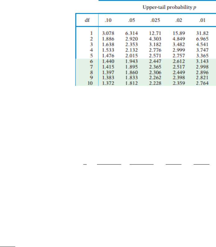
55
Table of Critical Values of t-Statistic
df= sample size-1= (n-1)
One can see that once the sample size starts exceeding 9-10 (df = 8, 9), the difference between the critical
values starts stabilizing. For example, for upper tail probability (= level of significance) of 0.05, the
difference between critical values for df = 9 and df =10 is only 0.021, where as the difference between
critical values for df= 4 and 5 is 0.117; similar patterns are noted for other levels of significance. For the
normal distribution, critical values used to compute UTL90-95, UTL95-95, USL90, and USL95 are
described as follows. One can see that once the sample size starts exceeding 9-10, the difference between
the critical values starts decreasing significantly.
n
UTL90-95
UTL95-95
USL90
USL95
3
6.155
7.656
1.148
1.153
4
4.162
5.144
1.425
1.462
5
3.407
4.203
1.602
1.671
6
3.006
3.708
1.729
1.822
7
2.755
3.399
1.828
1.938
8
2.582
3.187
1.909
2.032
9
2.454
3.031
1.977
2.11
10
2.355
2.911
2.036
2.176
11
2.275
2.815
2.088
2.234
Note: Nonparametric upper limits (UPLs, UTLs, and USLs) are computed using higher order statistics of
a data set. To achieve the desired confidence coefficient, samples of sizes much greater than 10 are
required. For details, refer to Chapter 3. It should be noted that critical values of USLs are significantly
lower than critical values for UTLs. Critical values associated with UTLs decrease as the sample size
increases. Since, as the sample size increases the maximum of the data set also increases, and critical
values associated with USLs increase with the sample size.
1.7.2 Sample Sizes for Bootstrap Methods
Several nonparametric methods including bootstrap methods for computing UCL, UTL, and other limits
for both full-uncensored data sets and left-censored data sets with NDs are available in ProUCL 5.1.
Bootstrap resampling methods are useful when not too few (e.g., < 15-20) and not too many (e.g., > 500-
1000) observations are available. For bootstrap methods (e.g., percentile method, BCA bootstrap method,
bootstrap-t method), a large number (e.g., 1000, 2000) of bootstrap resamples are drawn with replacement
from the same data set. Therefore, to obtain bootstrap resamples with at least some distinct values (so that
statistics can be computed from each resample), it is suggested that a bootstrap method should not be used
when dealing with small data sets of sizes less than 15-20. Also, it is not necessary to bootstrap a large

56
data set of size greater than 500 or 1000; that is when a data set of a large size (e.g., > 500) is available,
there is no need to obtain bootstrap resamples to compute statistics of interest (e.g., UCLs). One can
simply use a statistical method on the original large data set.
Note: Rules-of-thumb about minimum sample size requirements described in this section are based upon
professional experience of the developers. ProUCL software is not a policy software. It is recommended
that the users/project teams/agencies make determinations about the minimum number of observations
and minimum number of detects that should be present in a data set before using a statistical method.
1.8 Statistical Analyses by a Group ID
The analyses of data categorized by a group ID variable such as: 1) Surface vs. Subsurface; 2) AOC1 vs.
AOC2; 3) Site vs. Background; and 4) Upgradient vs. Downgradient monitoring wells are common in
environmental applications. ProUCL 5.1 offers this option for data sets with and without NDs. The
Group Option provides a tool for performing separate statistical tests and for generating separate
graphical displays for each member/category of the group (samples from different populations) that may
be present in a data set. The graphical displays (e.g., box plots, quantile-quantile plots) and statistics (e.g.,
background statistics, UCLs, hypotheses tests) of interest can be computed separately for each group by
using this option. Moreover, using the Group Option, graphical methods can display multiple graphs
(e.g., Q-Q plots) on the same graph providing graphical comparison of multiple groups.
It should be pointed out that it is the user’s responsibility to provide an adequate amount of data to
perform the group operations. For example, if the user desires to produce a graphical Q-Q plot (e.g., using
only detected data) with regression lines displayed, then there should be at least two detected data values
(to compute slope, intercept, sd) in the data set. Similarly, if the graphs are desired for each group
specified by the group ID variable, there should be at least two observations in each group specified by
the group variable. When ProUCL data requirements are not met, ProUCL does not perform any
computations, and generates a warning message (colored orange) in the lower Log Panel of the output
screen of ProUCL 5.1.
1.9 Statistical Analyses for Many Constituents/Variables
ProUCL software can process multiple analytes/variables simultaneously in a user-friendly manner This
option is useful when one has to process multiple variables and compute decision statistics (e.g., UCLs,
UPLs, and UTLs) and test statistics (e.g., ANOVA test, trend test) for multiple variables. It is the user’s
responsibility to make sure that each selected variable has an adequate amount of data so that ProUCL
can perform the selected statistical method correctly. ProUCL displays warning messages when a selected
variable does not have enough data needed to perform the selected statistical method.
1.10 Use of Maximum Detected Value as Estimates of Upper Limits
Some practitioners use the maximum detected value as an estimate of the EPC term. This is especially
true when the sample size is small such as < 5, or when a UCL95 exceeds the maximum detected values
(EPA 1992a). Also, many times in practice, the BTVs and not-to-exceed values are estimated by the
maximum detected value (e.g., nonparametric UTLs, USLs).
57
1.10.1 Use of Maximum Detected Value to Estimate BTVs and Not-to-Exceed Values
BTVs and not-to-exceed values represent upper threshold values from the upper tail of a data distribution;
therefore, depending upon the data distribution and sample size, the BTVs and other not-to-exceed values
may be estimated by the largest or the second largest detected value. A nonparametric UPL, UTL, and
USL are often estimated by higher order statistics such as the maximum value or the second largest value
(EPA 1992b, 2009, Hahn and Meeker 1991). The use of higher order statistics to estimate the UTLs
depends upon the sample size. For data sets of size: 1) 59 to 92 observations, a nonparametric UTL95-95
is given by the maximum detected value; 2) 93 to 123 observations, a nonparametric UTL95-95 is given
by the second largest maximum detected value; and 3) 124 to 152 observations, a UTL95-95 is given by
the third largest detected value in the sample, and so on.
1.10.2 Use of Maximum Detected Value to Estimate EPC Terms
Some practitioners tend to use the maximum detected value as an estimate of the EPC term. This is
especially true when the sample size is small such as < 5, or when a UCL95 exceeds the maximum
detected value. Specifically, the EPA (1992a) document suggests the use of the maximum detected value
as a default value to estimate the EPC term when a 95% UCL (e.g., the H-UCL) exceeds the maximum
value in a data set. ProUCL computes 95% UCLs of the mean using several methods based upon normal,
gamma, lognormal, and non-discernible distributions. In the past, a lognormal distribution was used as the
default distribution to model positively skewed environmental data sets. Additionally, only two methods
were used to estimate the EPC term based upon: 1) normal distribution and Student’s t-statistic, and 2)
lognormal distribution and Land’s H-statistic (Land 1971, 1975). The use of the H-statistic often yields
unstable and impractically large UCL95 of the mean (Singh, Singh, and Engelhardt 1997; Singh, Singh,
and Iaci 2002). For highly skewed data sets of smaller sizes (< 30, < 50), H-UCL often exceeds the
maximum detected value. Since the use of a lognormal distribution has been quite common (suggested as
a default model in the risk assessment guidance for Superfund [RAGS] document [EPA 1992a]), the
exceedance of the maximum value by an H-UCL95 is frequent for many skewed data sets of smaller sizes
(e.g., < 30, < 50). These occurrences result in the possibility of using the maximum detected value as an
estimate of the EPC term.
It should be pointed out that in some cases, the maximum observed value actually might represent an
impacted location. Obviously, it is not desirable to use an observation potentially representing an
impacted location to estimate the EPC for an AOC. The EPC term represents the average exposure
contracted by an individual over an EA during a long period of time; the EPC term should be estimated
by using an average value (such as an appropriate 95% UCL of the mean) and not by the maximum
observed concentration. One needs to compute an average exposure and not the maximum exposure.
Singh and Singh (2003) studied the performance of the max test (using the maximum observed value to
estimate the EPC) via Monte Carlo simulation experiments. They noted that for skewed data sets of small
sizes (e.g., < 10-20), even the max test does not provide the specified 95% coverage to the population
mean, and for larger data sets it overestimates the EPC term, which may lead to unnecessary further
remediation.
Several methods, some of which are described in EPA (2002a) and other EPA documents, are available in
versions of ProUCL (i.e., ProUCL 3.00.02 [EPA 2004], ProUCL 4.0 [U.S. EPA 2007], ProUCL 4.00.05
[EPA 2009, 2010], ProUCL 4.1 [EPA 2011]) for estimating the EPC terms. For data sets with NDs,
ProUCL 5.0 (and ProUCL 5.1) has some new UCL (and other limits) computation methods which were
not available in earlier versions of ProUCL. It is unlikely that the UCLs based upon those methods will
exceed the maximum detected value, unless some outliers are present in the data set.

58
1.10.2.1 Chebyshev Inequality Based UCL95
ProUCL 5.1 (and its earlier versions) displays a warning message when the suggested 95% UCL (e.g.,
Hall’s or bootstrap-t UCL with outliers) of the mean exceeds the detected maximum concentration. When
a 95% UCL does exceed the maximum observed value, ProUCL suggests the use of an alternative UCL
computation method based upon the Chebyshev inequality. One may use a 97.5% or 99% Chebyshev
UCL to estimate the mean of a highly skewed population. The use of the Chebyshev inequality to
compute UCLs tends to yield more conservative (but stable) UCLs than other methods available in
ProUCL software. In such cases, when the sample size is large (and other UCL methods such as the
bootstrap-t method yield unrealistically high values due to presence of outliers), one may want to use a
95% Chebyshev UCL or a Chebyshev UCL with a lower confidence coefficient such as 90% as an
estimate of the population mean, especially when the sample size is large (e.g., >100, 150). The details (as
functions of sample size and skewness) for the use of those UCLs are summarized in various versions of
ProUCL Technical Guides (EPA 2004, 2007, 2009, 2010d, 2011, 2013a).
Notes: Using the maximum observed value to estimate the EPC term representing the average exposure
contracted by an individual over an EA is not recommended. For the sake of interested users, ProUCL
displays a warning message when the recommended 95% UCL (e.g., Hall’s bootstrap UCL) of the mean
exceeds the observed maximum concentration. For such scenarios (when a 95% UCL does exceed the
maximum observed value), an alternative UCL computation method based upon Chebyshev inequality is
suggested by the ProUCL software.
1.11 Samples with Nondetect Observations
ND observations are inevitable in most environmental data sets. Singh, Maichle, and Lee (2006) studied
the performances (in terms of coverages) of the various UCL95 computation methods including the
simple substitution methods (such as the DL/2 and DL methods) for data sets with ND observations. They
concluded that the UCLs obtained using the substitution methods, including the replacement of NDs by
DL/2; do not perform well even when the percentage of ND observations is low, such as less than 5% to
10%. They recommended avoiding the use of substitution methods for computing UCL95 based upon
data sets with ND observations.
1.11.1 Avoid the Use of the DL/2 Substitution Method to Compute UCL95
Based upon the results of the report by Singh, Maichle, and Lee (2006), it is recommended to avoid the
use of the DL/2 substitution method when performing a GOF test, and when computing the summary
statistics and various other limits (e.g., UCL, UPL, UTLs) often used to estimate the EPC terms and
BTVs. Until recently, the substitution method has been the most commonly used method for computing
various statistics of interest for data sets which include NDs. The main reason for this has been the lack of
the availability of the other rigorous methods and associated software programs that can be used to
estimate the various environmental parameters of interest. Today, several methods (e.g., using KM
estimates) with better performance, including the Chebyshev inequality and bootstrap methods, are
available for computing the upper limits of interest. Several of those parametric and nonparametric
methods are available in ProUCL 4.0 and higher versions. The DL/2 method is included in ProUCL for
historical reasons as it had been the most commonly used and recommended method until recently (EPA
2006b). EPA scientists and several reviewers of the ProUCL software had suggested and requested the
inclusion of the DL/2 substitution method in ProUCL for comparison and research purposes.

59
Notes: Even though the DL/2 substitution method has been incorporated in ProUCL, its use is not
recommended due to its poor performance. The DL/2 substitution method has been retained in ProUCL
5.1 for historical and comparison purposes. NERL-EPA, Las Vegas strongly recommends avoiding the
use of this method even when the percentage of NDs is as low as 5% to 10%.
1.11.2 ProUCL Does Not Distinguish between Detection Limits, Reporting limits, or
Method Detection Limits
ProUCL 5.1 (and all previous versions) does not make distinctions between method detection limits
(MDLs), adjusted MDLs, sample quantitation limits (SQLs), reporting limits (RLs), or DLs. Multiple
DLs (or RLs) in ProUCL mean different values of the detection limits. It is user’s responsibility to
understand the differences between these limits and use appropriate values (e.g., DLs) for nondetect
values below which the laboratory cannot reliably detect/measure the presence of the analyte in collected
samples (e.g., soil samples). A data set consisting of values less than the DLs (or MDLs, RLs) is
considered a left-censored data set. ProUCL uses statistical methods available in the statistical literature
for left-censored data sets for computing statistics of interest including mean, sd, UCL, and estimates of
BTVs.
The user determines which qualifiers (e.g., J, U, UJ) will be considered as nondetects. Typically, all
values with U or UJ qualifiers are considered as nondetect values. It is the user's responsibility to enter a
value which can be used to represent a ND value. For NDs, the user enters the associated DLs or RLs
(and not zeros or half of the detection limits). An indicator column/variable, D_x taking a value, 0, for all
nondetects and a value, 1, for all detects is assigned to each variable, x, with NDs. It is the user’s
responsibility to supply the numerical values for NDs (should be entered as reported DLs) not qualifiers
(e.g., J, U, B, UJ). For example, for thallium with nondetect values, the user creates an associated column
labeled as D_thallium to tell the software that the data set will have nondetect values. This column,
D_thallium consists of only zeros (0) and ones (1); zeros are used for all values reported as NDs and ones
are used for all values reported as detects.
1.12 Samples with Low Frequency of Detection
When all of the sampled values are reported as NDs, the EPC term and other statistical limits should also
be reported as a ND value, perhaps by the maximum RL or the maximum RL/2. The project team will
need to make this determination. Statistics (e.g., UCL95) based upon only a few detected values (e.g., <
4) cannot be considered reliable enough to estimate EPCs which can have a potential impact on human
health and the environment. When the number of detected values is small, it is preferable to use ad hoc
methods rather than using statistical methods to compute EPCs and other upper limits. Specifically, for
data sets consisting of < 4 detects and for small data sets (e.g., size < 10) with low detection frequency
(e.g., < 10%), the project team and the decision makers should decide, on a site-specific basis, how to
estimate the average exposure (EPC) for the constituent and area under consideration. For data sets with
low detection frequencies, other measures such as the median or mode represent better estimates (with
lesser uncertainty) of the population measure of central tendency.
Additionally, when most (e.g., > 95%) of the observations for a constituent lie below the DLs, the sample
median or the sample mode (rather than the sample average) may be used as an estimate of the EPC. Note
that when the majority of the data are NDs, the median and the mode may also be represented by a ND
value. The uncertainty associated with such estimates will be high. The statistical properties, such as the
bias, accuracy, and precision of such estimates, would remain unknown. In order to be able to compute
defensible estimates, it is always desirable to collect more samples.
60
1.13 Some Other Applications of Methods in ProUCL 5.1
In addition to performing background versus site comparisons for CERCLA and RCRA sites, performing
trend evaluations based upon time-series data sets, and estimating EPCs in exposure and risk evaluation
studies, the statistical methods in ProUCL can be used to address other issues dealing with environmental
investigations that are conducted at Superfund or RCRA sites.
1.13.1 Identification of COPCs
Risk assessors and remedial project managers (RPMs) often use screening levels or BTVs to identify
COPCs during the screening phase of a cleanup project at a contaminated site. The screening for COPCs
is performed prior to any characterization and remediation activities that are conducted at the site. This
comparison is performed to screen out those constituents that may be present in the site medium of
interest at low levels (e.g., at or below the background levels or some pre-established screening levels)
and may not pose any threat and concern to human health and the environment. Those constituents may
be eliminated from all future site investigations, and risk assessment and risk management studies.
To identify the COPCs, point-by-point site observations are compared with some pre-established soil
screening levels (SSL) or estimated BTVs. This is especially true when the comparisons of site
concentrations with screening levels or BTVs are conducted in real time by the sampling or cleanup crew
onsite. The project team should decide the type of site samples (discrete or composite) and the number of
site observations that should be collected and compared with the screening levels or the BTVs. In case
BTVs or screening levels are not known, the availability of a defensible site-specific background or
reference data set of reasonable size (e.g., at least 10) is required for computing reliable and
representative estimates of BTVs and screening levels. The constituents with concentrations exceeding
the respective screening values or BTVs may be considered COPCs, whereas constituents with
concentrations (e.g., in all collected samples) lower than the screening values or BTVs may be omitted
from all future evaluations.
1.13.2 Identification of Non-Compliance Monitoring Wells
In MW compliance assessment applications, individual (often discrete) constituent concentrations from a
MW are compared with some pre-established limits such as an ACL or a maximum concentration limit
(MCL). An exceedance of the MCL or the BTV (e.g., estimated by a UTL95-95 or a UPL95) by a MW
concentration may be considered an indication of contamination in that MW. For individual concentration
comparisons, the presence of contamination (determined by an exceedance) may have to be confirmed by
re-sampling from that MW. If concentrations of constituents in the original sample and re-sample(s)
exceed the MCL or BTV, then that MW may require further scrutiny, perhaps triggering remediation
activities. If the concentration data from a MW for 4 to 5 continuous quarters (or some other designated
time period determined by the project team) are below the MCL or BTV level, then that MW may be
considered as complying with (achieving) the pre-established or estimated standards.
1.13.3 Verification of the Attainment of Cleanup Standards, C
s
Hypothesis testing approaches are used to verify the attainment of the cleanup standard, C
s
, at site AOCs
after conducting remediation and cleanup at those site AOCs (EPA 1989a, 1994). In order to assess the
attainment of cleanup levels, a representative data set of adequate size perhaps obtained using the DQO
process (or a minimum of 10 observations should be collected) needs to be made available from the
remediated/excavated areas of the site under investigation. The sample size should also account for the
61
size of the remediated site areas: meaning that larger site areas should be sampled more (with more
observations) to obtain a representative sample of the remediated areas under investigation. Typically, the
null hypothesis of interest is H
0
: Site Mean,
s
≥ C
s
versus the alternative hypothesis, H
1
: Site Mean,
s
<
C
s,
where the cleanup standard, C
s
, is known a priori.
1.13.4 Using BTVs (Upper Limits) to Identify Hot Spots
The use of upper limits (e.g., UTLs) to identify hot spot(s) has also been mentioned in the Guidance for
Comparing Background and Chemical Concentrations in Soil for CERCLA Sites (EPA 2002b). Point-by-
point site observations are compared with a pre-established or estimated BTV. Exceedances of the BTV
by site observations may represent impacted locations with elevated concentrations (hot spots).
1.14 Some General Issues, Suggestions and Recommendations made by
ProUCL
Some general issues regarding the handling of multiple DLs by ProUCL and recommendations made
about various substitution and ROS methods for data sets with NDs are described in the following
sections.
1.14.1 Handling of Field Duplicates
ProUCL does not pre-process field duplicates. The project team determines how field duplicates will be
handled and pre-processes the data accordingly. For an example, if the project team decides to use
average values for field duplicates, then averages need to be computed and field duplicates need to be
replaced by their respective average values. It is the user's responsibility to feed in appropriate values
(e.g., averages, maximum) for field duplicates. The user is advised to refer to the appropriate EPA
guidance documents related to collection and use of field duplicates for more information.
1.14.2 ProUCL Recommendation about ROS Method and Substitution (DL/2) Method
For data sets with NDs, ProUCL can compute point estimates of population mean and standard deviation
using the KM and ROS methods (and also using the DL/2 substitution method). The substitution method
has been retained in ProUCL for historical and research purposes. ProUCL uses Chebyshev inequality,
bootstrap methods, and normal, gamma, and lognormal distribution based equations on KM (or ROS)
estimates to compute upper limits (e.g., UCLs, UTLs). The simulation study conducted by Singh,
Maichle and Lee (2006) demonstrated that the KM method yields accurate estimates of the population
mean. They also demonstrated that for moderately skewed to highly skewed data sets, UCLs based upon
KM estimates and BCA bootstrap (mild skewness), KM estimates and Chebyshev inequality (moderate to
high skewness), and KM estimates and bootstrap-t method (moderate to high skewness) yield better (in
terms of coverage probability) estimates of EPCs than other UCL methods based upon the Student's t-
statistic on KM estimates, percentile bootstrap method on KM or ROS estimates.
1.14.3 Unhandled Exceptions and Crashes in ProUCL
A typical statistical software, especially developed under limited resources may not be able to
accommodate data sets with all kinds of deficiencies such as all missing values for a variable, or all
nondetect values for a variable. An inappropriate/insufficient data set can occur in various forms and not
all of them can be addressed in a scientific program like ProUCL. Specifically, from a programming point
of view, it can be quite burdensome on the programmer to address all potential deficiencies that can occur

62
in a data set. ProUCL 5.1 addresses many data deficiencies and produces warming messages. All data
deficiencies causing unhandled exceptions which were identified by users have been addressed in
ProUCL 5.1. However, when ProUCL yields an unhandled exception or crashes, it is highly likely that
there is something wrong with the data set; the user is advised to review the input data set to make sure
that the data set follows ProUCL data and formatting requirements.
1.15 The Unofficial User Guide to ProUCL4 (Helsel and Gilroy 2012)
Several ProUCL 4.1 users sent inquiries about the validity of the comments made about the ProUCL
software in the Unofficial User Guide to ProUCL4 (Helsel and Gilroy, 2012) and in the Practical Stats
webinar, "ProUCL v4: The Unofficial User Guide," presented by Dr. Helsel on October 15, 2012 (Helsel
2012a). Their inquiries led us to review comments made about the ProUCL4 software and its associated
guidance documents (EPA 2007, 2009a, 2009b, 2010c, 2010d, and 2011) in the “The Unofficial Users
Guide to ProUCL4” and in the webinar, "ProUCL v4: The Unofficial User Guide". These two documents
collectively are referred to as the Unofficial ProUCLv4 User Guide in this ProUCL document. The pdf
document describing the material presented in the Practical Stats Webinar (Helsel 2012a) was
downloaded from the http://www.practicalstats.com website.
In the "ProUCL v4: The Unofficial User Guide", comments have been made about the software and its
guidance documents, therefore, it is appropriate to address those comments in the present ProUCL
guidance document. It is necessary to provide the detailed response to assure that: 1) rigorous statistical
methods are used to compute decision making statistics; and 2) the methods incorporated in ProUCL
software are not misrepresented and misinterpreted. Some general responses and comments about the
material presented in the webinar and in the Unofficial User Guide to ProUCLv4 are described as follows.
Specific comments and responses are also considered in the respective chapters of ProUCL 5.1 (and
ProUCL 5.0) guidance documents.
Note: It is noted that the Kindle version of "ProUCL v4: Unofficial User Guide" is no longer available on
Amazon. Several incorrect theoretical statements and statements misrepresenting ProUCL 4 were made in
that Unofficial User Guide; therefore, a brief response to some of those statements has been retained in
ProUCL 5.1 guidance documents.
ProUCL is a freeware software package which has been developed under limited government funding to
address statistical issues associated with various environmental site projects. Not all statistical methods
(e.g., Levene test) described in the statistical literature have been incorporated in ProUCL. One should not
compare ProUCL with commercial software packages which are expensive and not as user-friendly as the
ProUCL software when addressing environmental statistical issues. The existing and some new statistical
methods based upon the research conducted by ORD-NERL, EPA Las Vegas during the last couple of
decades have been incorporated in ProUCL to address the statistical needs of various environmental site
projects and research studies. Some of those new methods may not be available in text books, in the
library of programs written in R-script, and in commercial software packages. However, those methods
are described in detail in the cited published literature and also in the ProUCL Technical Guides (e.g.,
EPA 2007, 2009a, 2009b, 2010c, 2010d, and 2011). Even though for uncensored data sets, programs
which compute gamma distribution based UCLs and UPLs are available in R Script, programs which
compute a 95% UCL of mean based upon a gamma distribution on KM estimates are not as easily
available.
In the Unofficial ProUCL v4 User Guide, several statements have been made about percentiles. There
are several ways to compute percentiles. Percentiles computed by ProUCL may or may not be

63
identical (don't have to be) to percentiles computed by NADA for R (Helsel 2013) or described in
Helsel and Gilroy (2012). To address users' requests, ProUCL 4.1 (2011) and its higher versions
compute percentiles that are comparable to the percentiles computed by Excel 2003 and higher
versions.
The literature search suggests that there are a total of nine (9) known types of percentiles, i.e., 9
different methods of calculating percentiles in statistics literature (Hyndman and Fan, 1996). The R
programming language (R Core Team 2012) computes percentiles using those 9 methods using the
following statement in R
Quantile (x, p, type=k) where p = percentile, k = integer between 1 - 9
ProUCL computes percentiles using Type 7; Minitab 16 and SPSS compute percentiles using Type 6.
It is simply a matter of choice, as there is no 'best' type to use. Many software packages use one type
for calculating a percentile, and another for generating a box plot (Hyndman and Fan 1996).
An incorrect statement "By definition, the sample mean has a 50% chance of being below the true
population mean" has been made in Helsel and Gilroy (2012) and also in Helsel (2012a). The above
statement is not correct for means of skewed distributions (e.g., lognormal or gamma) commonly
occurring in environmental applications. Since Helsel (2012) prefers to use a lognormal distribution,
the incorrectness of the above statement has been illustrated using a lognormal distribution. The
mean and median of a lognormal distribution (details in Section 2.3.2 of Chapter 2 of ProUCL 5.1
Technical Guide) are given by:
mean =
)5.0exp(
2
1
σμμ
; and median =
)exp(μM
From the above equations, it is clear that the mean of a lognormal distribution is always greater than
the median for all positive values of σ (sd of log-transformed variable). Actually the mean is greater
than the p
th
percentile when σ >2z
p
. For example, when p = 0.80, z
p
= 0.845, and mean of a
lognormal distribution, μ
1
exceeds x
0.80
, the 80
th
percentile when σ > 1.69. In other words, when σ >
1.69 the lognormal mean will exceed the 80
th
percentile of a lognormal distribution. Here z
p
represents the p
th
percentile of the standard normal distribution (SND) with mean 0 and variance 1.
To demonstrate the incorrectness of the above statement, a small simulation study was conducted.
The distribution of sample means based upon samples of size 100 were generated from lognormal
distributions with µ =4, and varying skewness. The experiment was performed 10,000 times to
generate the distributions of sample means. The probabilities of sample means less than the
population means were computed. The following results are noted.
Table 1-2. Probabilities
1
()px
Computed for Lognormal Distributions with µ=4 and Varying Values of σ
Results are based upon 10000 Simulation Runs for Each Lognormal Distribution Considered
Parameter
µ=4, σ=0.5
µ
1
=61.86
σ
1
=32.97
µ=4, σ=1
µ
1
=90.017
σ
1
=117.997
µ=4,σ=1.5
µ
1
=168.17
σ
1
=489.95
µ=4,σ=2
µ
1
=403.43
σ
1
=2953.53
µ=4,σ=2.5
µ
1
=1242.65,
σ
1
=28255.23
1
()px
0.519
0.537
0.571
0.651
0.729
Mean
61.835
89.847
168.70
405.657
1193.67
Median
61.723
89.003
160.81
344.44
832.189

64
The probabilities summarized in the above table demonstrate that the statement about the mean
made in Helsel and Gilroy (2012) is incorrect.
Graphical Methods: Graphical methods are available in ProUCL as exploratory tools which can be
generated for both uncensored and left-censored data sets. Exploratory graphical methods are used to
understand possible patterns present in data sets and not to compute statistics used in the decision
making process. The Unofficial ProUCL Guide makes several comments about box plots and Q-Q
plots incorporated in ProUCL. The Unofficial ProUCL Guide states that all graphs with NDs are
incorrect. These statements are misleading and incorrect. The intent of the graphical methods in
ProUCL is exploratory for the purpose of gaining information (e.g., outliers, multiple populations,
data distribution, patterns, and skewness) about a data set. Based upon the data displayed (ProUCL
displays a message [e.g., as a sub-title] in this regard) on those graphs, all statistics shown on those
graphs generated by ProUCL are correct.
Box Plots: In statistical literature, one can find several ways to generate box plots. The practitioners
may have their own preferences to use one method over the other. All box plot methods including the
one in ProUCL convey the same information about the data set (outliers, mean, median, symmetry,
skewness). ProUCL uses a couple of development tools such as FarPoint spread (for Excel type input
and output operations) and ChartFx (for graphical displays); and ProUCL generates box plots using
the built-in box plot feature in ChartFx. For all practical and exploratory purposes, box plots in
ProUCL are equally good (if not better) as those available in the various commercial software
packages, for examining data distribution (skewed or symmetric), identifying outliers, and comparing
multiple groups (main objectives of box plots in ProUCL).
o As mentioned earlier, it is a matter of choice of using percentiles/quartiles to construct a box
plot. There is no 'best' method for constructing a box plot. Many software packages use one
method (out of 9 as specified above) for calculating a percentile, and another for constructing
a box plot (Hyndman and Fan 1996).
Q-Q plots: All Q-Q plots incorporated in ProUCL are correct and of high quality. In addition to
identifying outliers, Q-Q plots are also used to assess data distributions. Multiple Q-Q plots are useful
for performing point-by-point comparisons of grouped data sets, unlike box plots based upon the five-
point summary statistics. ProUCL has Q-Q plots for normal, lognormal, and gamma distributions -
not all of these graphical capabilities are directly available in other software packages such as NADA
for R (Helsel 2013). ProUCL offers several exploratory options for generating Q-Q plots for data sets
with NDs. Only detected outlying observations may require additional investigation; therefore, from
an exploratory point of view, ProUCL can generate Q-Q plots excluding all NDs (and other options).
Under this scenario there is no need to retain place holders (computing plotting positions used to
impute NDs) as the objective is not to impute NDs. To impute NDs, ProUCL uses ROS methods
(Gamma ROS and log ROS) requiring place holders; and ProUCL computes plotting positions for all
detects and NDs to generate a proper regression model which is used to impute NDs. Also for
comparison purposes, ProUCL can be used to generate Q-Q plots on data sets obtained by replacing
NDs by their respective DLs or DL/2s. In these cases, no NDs are imputed, and there is no need to
retain placeholders for NDs. On these Q-Q plots, ProUCL displays some relevant statistics which are
computed based upon the data displayed on those graphs.
Helsel (2012a) states that the Summary Statistics module does not display KM estimates and that
statistics based upon logged data are useless. Typically, estimates computed after processing the data

65
do not represent summary statistics. Therefore, KM and ROS estimates are not displayed in the
Summary Statistics module. These statistics are available in several other modules including the
UCL and BTV modules. At the request of several users, summary statistics are computed based upon
logged data. It is believed that the mean, median, or standard deviation of logged data do provide
useful information about data skewness and data variability.
To test for the equality of variances, the F-test, as incorporated in ProUCL, performs fairly well and
the inclusion of the Levene's (1960) test will not add any new capability to the ProUCL software.
Therefore, taking budget constraints into consideration, Levene's test has not been incorporated in the
ProUCL software.
o Although it makes sense to first determine if the two variances are equal or unequal, this is
not a requirement to perform a t-test. The t-distribution based confidence interval or test for
1
-
2
based on the pooled sample variance does not perform better than the approximate
confidence intervals based upon Satterthwaite's test. Hence testing for the equality of
variances is not required to perform a two-sample t-test. The use of Welch-Satterthwaite's or
Cochran's method is recommended in all situations (see Hayes 2005).
Helsel (2012a) suggests that imputed NDs should not be made available to the users. The developers
of ProUCL and other researchers like to have access to imputed NDs. As a researcher, for exploratory
purposes only, one may want to have access to imputed NDs to be used in exploratory advanced
methods such as multivariate methods including data mining, cluster and principal component
analyses. It is noted that one cannot easily perform exploratory methods on multivariate data sets with
NDs. The availability of imputed NDs makes it possible for researchers and scientists to identify
potential patterns present in complex multivariate data by using data mining exploratory methods on
those multivariate data sets with NDs. Additional discussion on this topic is considered in Chapter 4
of the ProUCL 5.1 Technical Guide.
o The statements summarized above should not be misinterpreted. One may not use parametric
hypothesis tests such as a t-test or a classical ANOVA on data sets consisting of imputed
NDs. These methods require further investigation as the decision errors associated with such
methods remain unquantified. There are other methods such as the Gehan and T-W tests in
ProUCL 5.0/ProUCL 5.1 which are better suited to perform two-sample hypothesis tests
using data sets with multiple detection limits.
Outliers: Helsel (2012a) and Helsel and Gilroy (2012) make several comments about outliers. The
philosophy (with input from EPA scientists) of the developers of ProUCL about the outliers in
environmental applications is that those outliers (unless they represent typographical errors) may
potentially represent impacted (site related or otherwise) locations or monitoring wells; and therefore
may require further investigation. Moreover, decision statistics such as a UCL95 based upon a data
set with outliers gets inflated and tends to represent those outliers instead of representing the
population average. Therefore, a few low probability outliers coming from the tails of the data
distribution may not be included in the computation of the decision making upper limits (UCLs,
UTLs), as those upper limits get distorted by outliers and tend not to represent the parameters they are
supposed to estimate.
o The presence of outliers in a data set tends to destroy the normality of the data set. In other
words, a data set with outliers can seldom (may be when outliers are mild, lying around the
border of the central and tail parts of a normal distribution) follow a normal distribution.
66
There are modern robust and resistant outlier identification methods (e.g., Rousseeuw and
Leroy 1987; Singh and Nocerino 1995) which are better suited to identify outliers present in a
data set; several of those robust outlier identification methods are available in the Scout 2008
version 1.0 (EPA 2009) software package.
o For both Rosner and Dixon tests, it is the data set (also called the main body of the data set)
obtained after removing the outliers (and not the data set with outliers) that needs to follow a
normal distribution (Barnett and Lewis 1994). Outliers are not known in advance. ProUCL
has normal Q-Q plots which can be used to get an idea about potential outliers (or mixture
populations) present in a data set. However, since a lognormal model tends to accommodate
outliers, a data set with outliers can follow a lognormal distribution; this does not imply that
the outlier which may actually represent an impacted/unusual location does not exist! In
environmental applications, outlier tests should be performed on raw data sets, as the cleanup
decisions need to be made based upon values in the raw scale and not in log-scale or some
other transformed space. More discussion about outliers can be found in Chapter 7 of the
ProUCL 5.1 Technical Guide.
In Helsel (2012a), it is stated, "Mathematically, the lognormal is simpler and easier to interpret than
the gamma (opinion)." We do agree with the opinion that the lognormal is simpler and easier to use
but the log-transformation is often misunderstood and hence incorrectly used and interpreted.
Numerous examples (e.g., Example 2-1 and 2-2, Chapter 2 of ProUCL Technical Guide) are provided
in the ProUCL guidance documents illustrating the advantages of the using a gamma distribution.
It is further stated in Helsel (2012a) that ProUCL prefers the gamma distribution because it
downplays outliers as compared to the lognormal. This argument can be turned around - in other
words, one can say that the lognormal is preferred by practitioners who want to inflate the effect of
the outlier. Setting this argument aside, we prefer the gamma distribution as it does not transform the
variable so the results are in the same scale as the collected data set. As mentioned earlier, log-
transformation does appear to be simpler but problems arise when practitioners are not aware of the
pitfalls (e.g., Singh and Ananda 2002; Singh, Singh, and Iaci 2002) associated with the use of
lognormal distribution.
Helsel (2012a) and Helsel and Gilroy (2012) state that "lognormal and gamma are similar, so usually
if one is considered possible, so is the other." This is another incorrect and misleading statement;
there are significant differences in the two distributions and in their mathematical properties. Based
upon the extensive experience in environmental statistics and published literature, for skewed data
sets that follow both lognormal and gamma distributions, the developers favor the use of the gamma
distribution over the lognormal distribution. The use of the gamma distribution based decision
statistics is preferred to estimate the environmental parameters (mean, upper percentile). A lognormal
model tends to hide contamination by accommodating outliers and multiple populations whereas a
gamma distribution tends not to accommodate contamination (elevated values) as can be seen in
Examples 2-1 and 2-2 of Chapter 2 of the ProUCL 5.1 Technical Guide. The use of the lognormal
distribution on a data set with outliers tends to yield inflated and distorted estimates which may not be
protective of human health and the environment; this is especially true for skewed data sets of small
of sizes <20-30; the sample size requirement increases with skewness.
o In the context of computing a UCL95 of mean, Helsel and Gilroy (2012) and Helsel (2012a) state
that GROS and LROS methods are probably never better than the KM method. It should be
noted that these three estimation methods compute estimates of mean and standard deviation and
67
not the upper limits used to estimate EPCs and BTVs. The use of the KM method does yield good
estimates of the mean and standard deviation as noted by Singh, Maichle, and Lee (2006). The
problem of estimating mean and standard deviation for data sets with nondetects has been studied
by many researchers as described in Chapter 4 of the ProUCL 5.1 Technical Guide. Computing
good estimates of mean and sd based upon left-censored data sets addresses only half of the
problem. The main issue is to compute decision statistics (UCL, UPL, UTL) which account for
uncertainty and data skewness inherently present in environmental data sets.
o Realizing that for skewed data sets, Student's t-UCL, CLT-UCL, and standard and percentile
bootstrap UCLs do not provide the specified coverage to the population mean for uncensored data
sets, many researchers (e.g., Johnson 1978; Chen 1995; Efron and Tibshirani 1993; Hall [1988,
1992]; Grice and Bain 1980; Singh, Singh, and Engelhardt 1997; Singh, Singh, and Iaci 2002)
developed parametric (e.g., gamma) and nonparametric (e.g., bootstrap-t and Hall's bootstrap
method, modified-t, and Chebyshev inequality) methods for computing confidence intervals and
upper limits which adjust for data skewness. One cannot ignore the work and findings of the
researchers cited above, and assume that Student's t-statistic based upper limits or percentile
bootstrap method based upper limits can be used for all data sets with varying skewness and
sample sizes.
o Analytically, it is not feasible to compare the various estimation and UCL computation methods
for skewed data sets containing ND observations. Instead, researchers use simulation
experiments to learn about the distributions and performances of the various statistics (e.g., KM-t-
UCL, KM-percentile bootstrap UCL, KM-bootstrap-t UCL, KM-Gamma UCL). Based upon the
suggestions made in published literature and findings summarized in Singh, Maichle, and Lee
(2006), it is reasonable to state and assume that the findings of the simulation studies performed
on uncensored skewed data sets comparing the performances of the various UCL computation
methods can be extended to skewed left-censored data sets.
o Like uncensored skewed data sets, for left-censored data sets, ProUCL 5.0/ProUCL 5.1 has
several parametric and nonparametric methods to compute UCLs and other limits which adjust
for data skewness. Specifically, ProUCL uses KM estimates in gamma equations; in the
bootstrap-t method, and in the Chebyshev inequality to compute upper limits for left-censored
skewed data sets.
Helsel (2012a) states that ProUCL 4 is based upon presuppositions. It is emphasized that ProUCL
does not make any suppositions in advance. Due to the poor performance of a lognormal model, as
demonstrated in the literature and illustrated via examples throughout ProUCL guidance documents,
the use of a gamma distribution is preferred when a data set can be modeled by a lognormal model
and a gamma model. To provide the desired coverage (as close as possible) for the population mean,
in earlier versions of ProUCL (version 3.0), in lieu of H-UCL, the use of Chebyshev UCL was
suggested for moderately and highly skewed data sets. In later (3.00.02 and higher) versions of
ProUCL, depending upon skewness and sample size, for gamma distributed data sets, the use of the
gamma distribution was suggested for computing the UCL of the mean.
Upper limits (e.g., UCLs, UPLs, UTLs) computed using the Student's t statistic and percentile bootstrap
method (Helsel 2012, NADA for R, 2013) often fail to provide the desired coverage (e.g., 95% confidence
coefficient) to the parameters (mean, percentile) of most of the skewed environmental populations. It is
suggested that the practitioners compute the decision making statistics (e.g., UCLs, UTLs) by taking: data

68
distribution; data set size; and data skewness into consideration. For uncensored and left-censored data
sets, several such upper limits computation methods are available in ProUCL 5.1 and its earlier versions.
Contrary to the statements made in Helsel and Gilroy (2012), ProUCL software does not favor statistics
which yield higher (e.g., nonparametric Chebyshev UCL) or lower (e.g., preferring the use of a gamma
distribution to using a lognormal distribution) estimates of the environmental parameters (e.g., EPC and
BTVs). The main objectives of the ProUCL software funded by the U.S. EPA is to compute rigorous
decision statistics to help the decision makers and project teams in making sound decisions which are
cost-effective and protective of human health and the environment.
Cautionary Note: Practitioners and scientists are cautioned about: 1) the suggestions made about the
computations of upper limits described in some recent environmental literature such as the NADA books
(Helsel [2005, 2012]); and 2) the misleading comments made about the ProUCL software in the training
courses offered by Practical Stats during 2012 and 2013. Unfortunately, comments about ProUCL made
by Practical Stats during their training courses lack professionalism and theoretical accuracy. It is noted
that NADA packages in R and Minitab (2013) developed by Practical Stats do not offer methods which
can be used to compute reliable or accurate decision statistics for skewed data sets. Decision statistics
(e.g., UCLs, UTLs, UPLs) computed using the methods (e.g., UCLs computed using percentile bootstrap,
and KM and LROS estimates and t-critical values) described in the NADA books and incorporated in
NADA packages do not take data distribution and data skewness into consideration. The use of statistics
suggested in NADA books and in Practical Stats training sessions often fail to provide the desired
specified coverage to environmental parameters of interest for moderately skewed to highly skewed
populations. Conclusions derived based upon those statistics may lead to incorrect conclusions which
may not be cost-effective or protective of human health and the environment.
Page 75 (Helsel [2012]): One of the reviewers of the ProUCL 5.0 software drew our attention to the
following incorrect statement made on page 75 of Helsel (2012):
"If there is only 1 reporting limit, the result is that the mean is identical to a substitution of the reporting
limit for censored observations."
An example of a left-censored data set containing ND observations with one reporting limit of 20 which
illustrates this issue is described as follows.
Y
D_y
20
0
20
0
20
0
7
1
58
1
92
1
100
1
72
1
11
1
27
1
The mean and standard deviation based upon the KM and two substitution methods: DL/2 and DL are
summarized as follows:

69
Kaplan-Meier (KM) Statistics
Mean 39.4
SD 35.56
DL Substitution method (replacing censored values by the reporting limit)
Mean 42.7
SD 34.77
DL/2 Substitution method (replacing NDs by the reporting limit)
Mean 39.7
SD 37.19
The above example illustrates that the KM mean (when only 1 detection limit is present) is not actually
identical to the mean estimate obtained using the substitution, DL (RL) method. The statement made in
Helsel's text (and also incorrectly made in his presentations such as the one made at the U.S. EPA 2007
National Association of Regional Project Managers (NARPM) Annual Conference:
http://www.ttemidev.com/narpm2007Admin/conference/) holds only when all observations reported
as detects are greater than the single reporting limit, which is not always true for environmental data sets
consisting of analytical concentrations.
1.16 Box and Whisker Plots
At the request of ProUCL users, a brief description of box plots (also known as box and whisker plots) as
developed by Tukey (Hoaglin, Mosteller and Tukey 1991) is provided in this section. A box and
whiskers plot represents a useful and convenient exploratory tool and provides a quick five-point
summary of a data set. In statistical literature, one can find several ways to generate box plots. The
practitioners may have their own preferences to use one method over the other. Box plots are well
documented in the statistical literature and description of box plots can be easily obtained by surfing the
net. Therefore, the detailed description about the generation of box plots is not provided in ProUCL
guidance documents. ProUCL also generates box plots for data set with NDs. Since box plots are used
for exploratory purposes to identify outliers and also to compare concentrations of two or more groups, it
does not really matter how NDs are displayed on those box plots. ProUCL generates box plots using
detection limits and draws a horizontal line at the highest detection limit. Users can draw up to four
horizontal lines at other levels (e.g., a screening level, a BTV, or an average) of their choice.
All box plot methods, including the one in ProUCL, represent five-point summary graphs including: the
lowest and the highest data values, median (50
th
percentile=second quartile, Q2), 25
th
percentile (lower
quartile, Q1), and 75
th
percentile (upper quartile, Q3). A box and whisker plot also provides information
about the degree of dispersion (interquartile range (IQR) = Q3-Q1=length/height of the box in a box plot),
the degree of skewness (suggested by the length of the whiskers) and unusual data values known as
outliers. Specifically, ProUCL (and other software packages) use the following to generate a box and
whisker plot.
Q1= 25
th
percentile, Q2= 50
th
(median), and Q3 = 75
th
percentile
Interquartile range= IQR = Q3-Q1 (the length/height of the box in a box plot)
Lower whisker starts at Q1 and the upper whisker starts at Q3.
Lower whisker extends up to the lowest observation or (Q1 - 1.5 * IQR) whichever is higher
Upper whisker extends up to the highest observation or (Q3 + 1.5 * IQR) whichever is lower
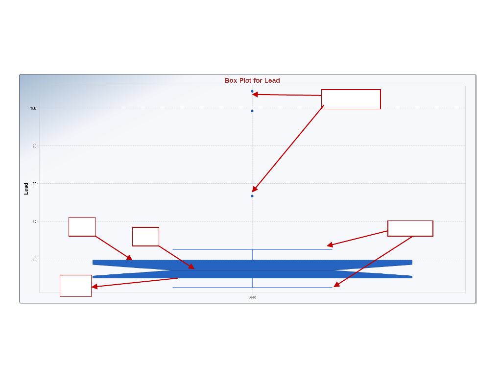
70
Horizontal bars (also known as fences) are drawn at the end of whiskers
Guidance in statistical literature suggests that observations lying outside the fences (above the
upper bar and below the lower bar) are considered potential outliers
An example box plot generated by ProUCL is shown in the following graph.
Box Plot with Fences and Outlier
It should be pointed out that the use of box plots in different scales (e.g., raw-scale and log-scale) may
lead to different conclusions about outliers. Below is an example illustrating this issue.
Example 1-2. Consider an actual data set consisting of copper concentrations collected a Superfund Site.
The data set is: 0.83, 0.87, 0.9, 1, 1, 2, 2, 2.18, 2.73, 5, 7, 15, 22, 46, 87.6, 92.2, 740, and 2960. Box plots
using data in the raw-scale and log-scale are shown in Figures 1-1 and 1-2.
Outliers
Fences
Q3
Q1
Q2
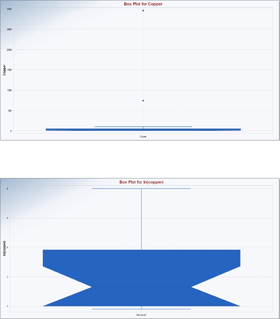
71
Figure 1-1. Box Plot of Raw Data in Original Scale
Based upon the last bullet point of the description of box plots described above, from Figure 1-1, it is
concluded that two observations 740 and 2960 in the raw scale represent outliers.
Figure 1-2. Box Plot of Data in Log-Scale
However, based upon the last bullet point about box plots, from Figure 1-2, it is concluded that two
observations 740 and 2960 in the log-scale do not represent outliers. The log-transformation has
accommodated the two outliers. This is one of the reasons ProUCL guidance suggests avoiding the use of
log-transformed data. The use of a log-transformation tends to hide/accommodate outliers/contamination.

72
Note: ProUCL uses a couple of development tools such as FarPoint spread (for Excel type input and
output operations) and ChartFx (for graphical displays). ProUCL generates box plots using the built-in
box plot feature in ChartFx. The programmer has no control over computing various statistics (e.g., Q1,
Q2, Q3, IQR) using ChartFx. So box plots generated by ProUCL can differ slightly from box plots
generated by other programs (e.g., Excel). However, for all practical and exploratory purposes, box plots
in ProUCL are equally good (if not better) as available in the various commercial software packages for
investigating data distribution (skewed or symmetric), identifying outliers, and comparing multiple
groups (main objectives of box plots).
Precision in Box Plots: Box plots generated using ChartFx round values to the nearest integer. For
increased precision of graphical displays (all graphical displays generated by ProUCL), the user can use
the process described as follows.
Position your cursor on the graph and right-click, a popup menu will appear. Position the cursor on
Properties and right-click; a windows form labeled Properties will appear. There are three choice at the
top: General, Series and Y-Axis. Position the e cursor over the Y-Axis choice and left-click. You can
change the number of decimals to increase the precision, change the step to increase or decrease the
number Y-Axis values displayed and/or change the direction of the label. To show values on the plot
itself, position your cursor on the graph and right-click; a pop-up menu will appear. Position the cursor on
Point Labels and right-click. There are other options available in this pop-up menu including changing
font sizes.
73
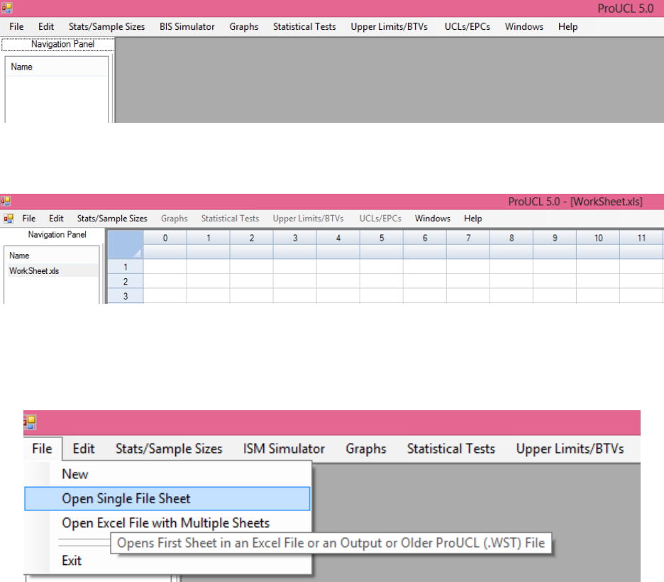
74
Chapter 2
Entering and Manipulating Data
2.1 Creating a New Data Set
By executing ProUCL 5.1, the following file options will appear (the title will show ProUCL 5.1 instead
of ProUCL 5.0):
By choosing the File ► New option, a new worksheet shown below will appear. The user enters variable
names and data following the ProUCL input file format requirements described in Section 2.3.
2.2 Opening an Existing Data Set
The user can open an existing worksheet (*.xls, *.xlsx, *.wst, and *.ost) by choosing the File ► Open
Single File Sheet option. The following drop down menu will appear:
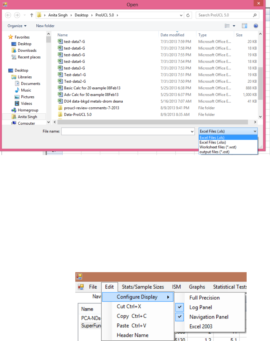
75
Choose a file by high lighting the type of file such as .xls as shown above. This option can also be used
to read in a *.wst worksheet and *.ost output sheet generated by earlier versions (e.g., ProUCL 4.1 and
older) of ProUCL.
By choosing the File ► Excel Multiple Sheets option, the user can open an Excel file consisting of
multiple sheets. Each sheet will be opened as a separate file to be processed individually by ProUCL 5.1
Caution: If you are editing a file (e.g., an excel file using Excel), make sure to close the file before
importing the file into ProUCL using the file open option.
2.3 Input File Format
The program can read Excel files. The user can perform typical Cut, Paste, and Copy
operations available under the Edit Menu Option as shown below.

76
The first row in all input data files consist of alphanumeric (strings of numbers and
characters) names representing the header row. Those header names may represent
meaningful variable names such as Arsenic, Chromium, Lead, Group-ID, and so on.
o The Group-ID column holds the labels for the groups (e.g., Background, AOC1, AOC2,
1, 2, 3, a, b, c, Site 1, Site 2) that might be present in the data set. Alphanumeric strings
(e.g., Surface, Sub-surface) can be used to label the various groups. Most of the modules
of ProUCL can process data by a group variable.
o The data file can have multiple variables (columns) with unequal numbers of
observations. Most of the modules of ProUCL can process data by a group variable.
o Except for the header row and columns representing the group labels, only numerical
values should appear in all other rows.
o All alphanumeric strings and characters (e.g., blank, other characters, and strings), and all
other values (that do not meet the requirements above) in the data file are treated as
missing values and are omitted from statistical evaluations.
o Also, a large value denoted by 1E31 (= 1x10
31
) can be used to represent missing data
values. All entries with this value are ignored from the computations. These values are
counted under the number of missing values.
2.4 Number Precision
The user may turn “Full Precision” on or off by choosing Configure ► Full Precision
On/OFF
By leaving “Full Precision” turned off, ProUCL will display numerical values using an
appropriate (default) decimal digit option; and by turning “Full Precision” off, all decimal
values will be rounded to the nearest thousandths place.
The “Full Precision” on option is specifically useful when dealing with data sets consisting of
small numerical values (e.g., < 1) resulting in small values of the various estimates and test
statistics. These values may become so small with several leading zeros (e.g., 0.00007332)
after the decimal. In such situations, one may want to use the "Full Precision” on option to
see nonzero values after the decimal.
Note: For the purpose of this User Guide, unless noted otherwise, all examples have used the “Full
Precision” OFF option. This option prints out results up to 3 significant digits after the decimal.
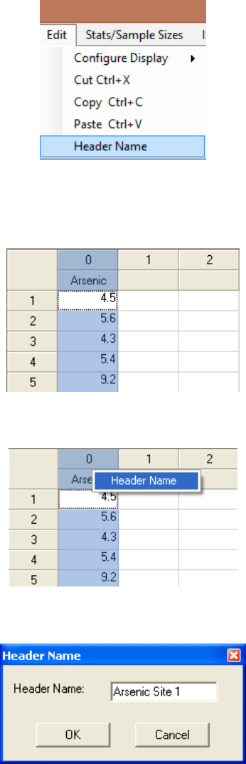
77
2.5 Entering and Changing a Header Name
1. The user can change variable names (Header Name) using the following process. Highlight the
column whose header name (variable name) you want to change by clicking either the column
number or the header as shown below.
2. Right-click and then click Header Name.
3. Change the Header Name.
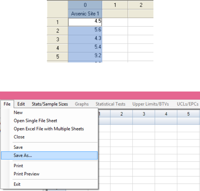
78
4. Click the OK button to get the following output with the changed variable name.
2.6 Saving Files
The Save option allows the user to save the active window in Excel 2003 or Excel 2007.
The Save As option also allows the user to save the active window. This option follows typical
Windows standards, and saves the active window to a file in .xls or .xlsx format. All
modified/edited data files, and output screens (excluding graphical displays) generated by the
software can be saved as .xls or .xlsx files.
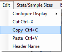
79
2.7 Editing
Click on the Edit menu item to reveal the following drop-down options.
Cut option: similar to a standard Windows Edit option, such as in Excel. It performs standard
edit functions on selected highlighted data (similar to a buffer).
Copy option: similar to a standard Windows Edit option, such as in Excel. It performs typical
edit functions on selected highlighted data (similar to a buffer).
Paste option: similar to a standard Windows Edit option, such as in Excel. It performs typical
edit functions of pasting the selected (highlighted) data to the designated spreadsheet cells or
area.
2.8 Handling Nondetect Observations and Generating Files with Nondetects
Several modules of ProUCL (e.g., Statistical Tests, Upper limits/BTVs, UCLs/EPCs) handle
data sets containing ND observations with single and multiple DLs.
The user informs the program about the status of a variable consisting of NDs. For a variable
with ND observations (e.g., arsenic), the detected values, and the numerical values of the
associated detection limits (for less than values) are entered in the appropriate column
associated with that variable. No qualifiers or flags (e.g., J, B, U, UJ, X) should be entered in
data files with ND observations.
Data for variables with ND values are provided in two columns. One column consists of
numerical values of detected observations and numerical values of detection limits (or
reporting limits) associated with observations reported as NDs; and the second column
represents their detection status consisting of only 0 (for ND values) and 1 (for detected
values) values. The name of the corresponding variable representing the detection status
should start with d_, or D_ (not case sensitive) and the variable name. The detection status
column with variable name starting with a D_ (or a d_) should have only two values: 0 for
ND values, and 1 for detected observations.
For example, the header name, D_Arsenic is used for the variable, Arsenic having ND
observations. The variable D_Arsenic contains a 1 if the corresponding Arsenic value
represents a detected entry, and contains a 0 if the corresponding entry represents a ND entry.
If this format is not followed, the program will not recognize that the data set has NDs. An
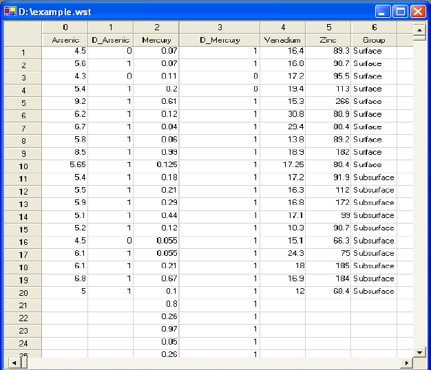
80
example data set illustrating these points is given as follows. ProUCL does not distinguish
between lowercase and uppercase letters.
2.9 Caution
Care should be taken to avoid any misrepresentation of detected and nondetected values.
Specifically, do not include any missing values (blanks, characters) in the D_column
(detection status column). If a missing value is located in the D_column (and not in the
associated variable column), the corresponding value in the variable column is treated as a
ND, even if this might not have been the intention of the user.
It is mandatory that the user makes sure that only a 1 or a 0 are entered in the detection status
D_column. If a value other than a 0 or a 1 (such as qualifiers) is entered in the D_ column
(the detection column), results may become unreliable, as the software defaults to any
number other than 0 or 1 as a ND value.
When computing statistics for full uncensored data sets without any ND values, the user
should select only those variables (from the list of available variables) that contain no ND
observations. Specifically, ND values found in a column chosen for the summary statistics
(full-uncensored data set) will be treated as a detected value; whatever value (e.g., detection
limit) is entered in that column will be used to compute summary statistics for a full-
uncensored data set without any ND values.
It is mandatory that the header name of a nondetect column associated with a variable such as
XYZ should be D_XYZ (or d_Xyz). No other characters or blanks are allowed. However, the
header (column) names are not case sensitive. If the nondetect column is not labeled properly,
methods to handle nondetect data will not be activated and shown.
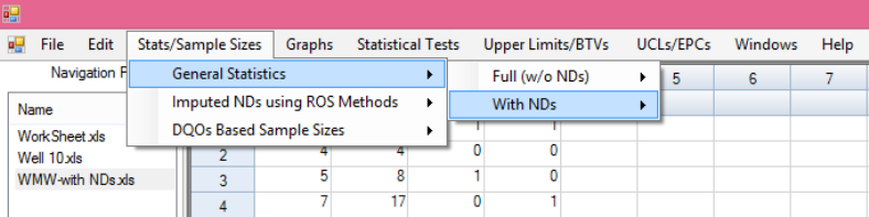
81
Two-Sample Hypotheses: When using two-sample hypotheses tests (WMW test, Gehan test,
and T-W test) on data sets with NDs, both samples or variables (e.g., site-As, Back-As)
should be specified as having NDs, even though one of the variables may not have any ND
observations. This means that a ND column (with 0 = ND, and 1 = detect) should be provided
for each variable (here D_site-As, and D_Back-As) to be used in this comparison. If a
variable (e.g., site-As) does not have any NDs, still a column with label D_site-As should be
included in the data set with all entries = 1 (detected values).
The sample data set given on the previous page illustrates points related to this option and
issues listed above. The data set contains some ND measurements for arsenic and mercury. It
should be noted that mercury concentrations are used to illustrate the points related to ND
observations; arsenic and zinc concentrations are used to illustrate the use of the group
variable, Group (Surface, Subsurface).
If for mercury, one computes summary statistics (assuming no ND values) using “Full” data
set option, then all ND values (with “0” entries in D_Mercury column) will be treated as
detected values, and summary statistics will be computed accordingly.
2.10 Summary Statistics for Data Sets with Nondetect Observations
To compute statistics of interest (e.g., background statistics, GOF test, UCLs, WMW test) for
variables with ND values, one should choose the ND option, With NDs, from the available
menu options such as Stats/Sample Sizes, Graphs, Statistical Tests, Upper Limits/BTVs,
and UCLs/EPCs.
The NDs option of these modules gets activated only when your data set contains NDs.
For data sets with NDs, the Stats/Sample Sizes module of ProUCL 5.0 computes summary
statistics and other general statistics such as the KM mean and KM standard deviation based
upon raw as well as log-transformed data.
The General Statistics/With NDs option also provides simple statistics (e.g., % NDs, Max
detect, Min detect, Mean) based upon detected values. The statistics computed in log-scale
(e.g., sd of log-transformed detected values) may help a user to determine the degree of
skewness (e.g., mild, moderate, high) of a data set based upon detected values. These
statistics may also help the user to choose the most appropriate method (e.g., KM bootstrap-t
UCL or KM percentile bootstrap UCL) to compute UCLs, UPLs, and other limits used to
compute decision statistics.
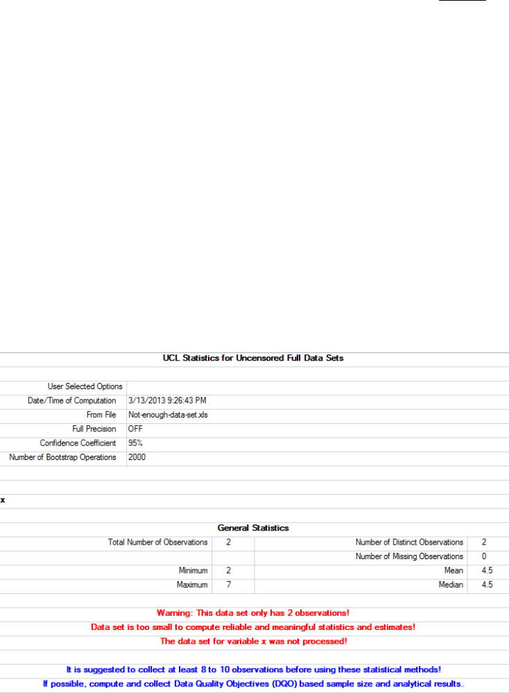
82
All other parametric and nonparametric statistics and estimates of population mean, variance,
percentiles (e.g., KM, and ROS estimates) for variables with ND observations are provided in
other menu options such as Upper Limits/BTVs and UCLs/EPCs.
2.11 Warning Messages and Recommendations for Data Sets with an
Insufficient Amount of Data
ProUCL provides warning messages and recommendations for data sets with an insufficient
amount of data for calculating meaningful estimates and statistics of interest. For example, it
is not desirable to compute an estimate of the EPC term based upon a discrete (as opposed to
composite or ISM) data set of size less than 5, especially when NDs are also present in the
data set.
However, to accommodate the computation of UCLs and other limits based upon ISM data
sets, ProUCL 5.0 allows users to compute UCLs, UPLs, and UTLs based upon data sets of
sizes as small as 3. The user is advised to follow the guidance provided in the ITRC ISM
Technical Regulatory Guidance Document (2012) to select an appropriate UCL95 to estimate
the EPC term. Due to lower variability in ISM data, the minimum sample size requirements
for statistical methods used on ISM data are lower than the minimum sample size
requirements for statistical methods used on discrete data sets.
It is suggested that for data sets composed of observations resulting from discrete sampling,
at least 10 observations should be collected to compute UCLs and various other limits.
Some examples of data sets with insufficient amount of data include data sets with less than 3
distinct observations, data sets with only one detected observation, and data sets consisting of
all nondetects.
Some of the warning messages generated by ProUCL 5.0 are shown as follows.
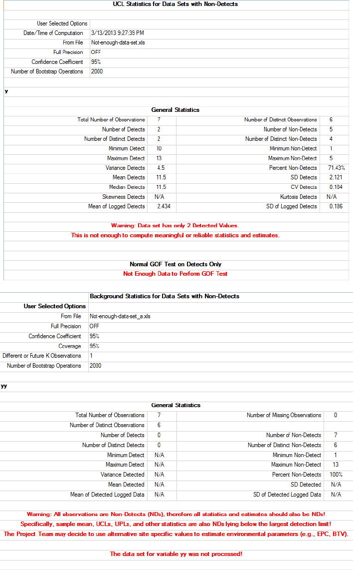
83
84
2.12 Handling Missing Values
The modules (e.g., Stats, GOF, UCLs, BTVs, Regression, Trend tests) of ProUCL 5.0 can
handle missing values within a data set. Appropriate messages are displayed when deemed
necessary.
All blanks, alphanumeric strings (except for group variables), or the specific large value 1e31
are considered as missing values.
A group variable (representing two or more groups, populations, MWs) can have
alphanumeric values (e.g., MW01, MW02, AOC1, AOC2).
ProUCL ignores all missing values in all statistical evaluations it performs. Missing values
are therefore not treated as being part of a data set.
Number of Valid Samples or Number of Valid Observations represents the Total Number of
Observations minus the Number of Missing Values. If there are no missing values, then
number of valid samples = total number of observations.
Valid Samples = Total Number of Observations – Missing Values.
It is important to note, however, that if a missing value not meant (e.g., a blank, or 1e31) to
represent a group category is present in a “Group” variable, ProUCL 5.1/ProUCL 5.0 will
treat that blank value (or 1e31 value) as a new group. All variables and values that correspond
to this missing value will be treated as part of a new group and not with any existing groups.
It is therefore important to check the consistency and validity of all data sets before
performing statistical evaluations.
ProUCL prints out the number of missing values (if any) and the number of reported values
(excluding the missing values) associated with each variable in the data sheet. This
information is provided in several output sheets (e.g., General statistics, BTVs, UCLs,
Outliers, OLS, Trend Tests) generated by ProUCL 5.1.
Number of missing values in Regression: The OLS module also handles the number of
missing values in the two columns (X and Y) representing independent (X) and dependent
(Y) variables. ProUCL provides warning messages for bad data sets (e.g., all identical
values) when statistics of interest cannot be computed. However, a bad/extreme data set can
occur in numerous different ways, and ProUCL may not cover all of those extreme/bad data
sets. In such cases, ProUCL may still yield an error message. The user needs to review and
fix his data set before performing regression or trend analysis again.
For further clarification of labeling missing values, the following example illustrates the terminology used
for the number of valid samples and of unique and distinct samples on output sheets generated by the
ProUCL software.
Example: The following example illustrates the notion of Valid Samples, Unique or Distinct Samples,
and Missing Values. The data set also has ND values. ProUCL 5.0 computes these numbers and prints
them on the UCLs and background statistics output.
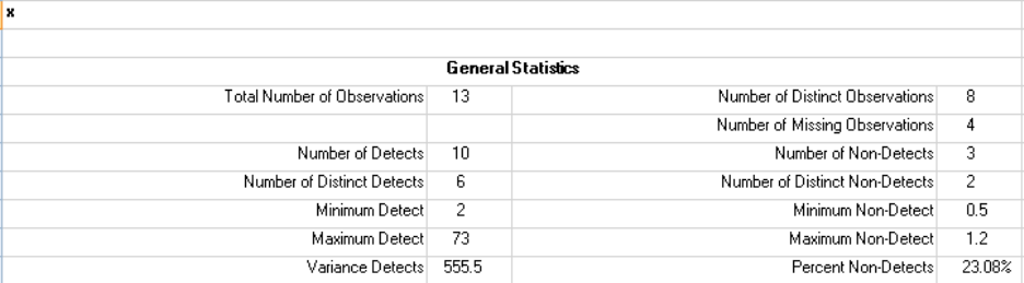
85
x D_x
2 1
4 1
2.3 1
1.2 0
w34 0
1.0E+031 0
0
anm 0
34 1
23 1
0.5 0
0.5 0
2.3 1
2.3 1
2.3 1
34 1
73 1
Valid Samples: Represents the total number of observations (censored and uncensored inclusive)
excluding the missing values. In this case the number of valid samples = 9. If a data set has no missing
value, then the total number of data points equals number of valid samples.
Missing Values: All values not representing a real numerical number are treated as missing values.
Specifically, all alphanumeric values including blanks are considered to be missing values. Big numbers
such as 1.0e31 are also treated as missing values and are considered as not valid observations. In the
example above the number of missing values = 4.
Unique or Distinct Samples: The number of unique samples or number of distinct samples represents all
unique (or distinct) detected and nondetected values. This is computed separately for detects and NDs.
This number is especially useful when using bootstrap methods. As well known, it is not desirable and
advisable to use bootstrap methods, when the number of unique samples is small. In the example above
total number of unique or distinct samples = 8, number of distinct detects = 6, and number of distinct NDs
(with different detection limits) = 2.
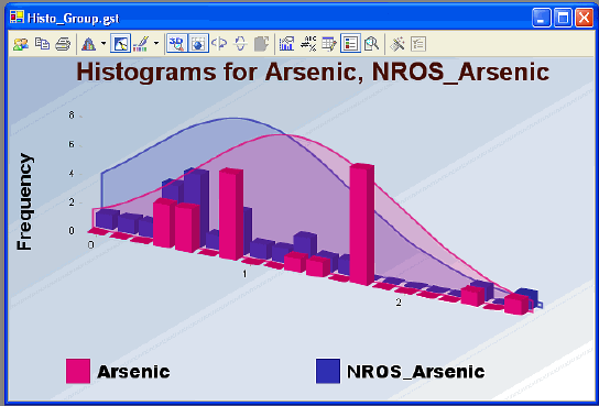
86
2.13 User Graphic Display Modification
Advanced users are provided two sets of tools to modify graphics displays. A graphics tool bar is
available above the graphics display; the user can right-click on the desired object within the graphics
display, and a drop-down menu will appear. The user can select an item from the drop-down menu list by
clicking on that item. This will allow the user to make modifications as available for the selected menu
item. An illustration is given as follows.
2.13.1 Graphics Tool Bar
The user can change fonts, font sizes, vertical and horizontal axis’s, select new colors for the various
features and text. All these actions are generally used to modify the appearance of the graphic display.
The user is cautioned that these tools can be unforgiving and may put the user in a situation where the
user cannot go back to the original display. Users are on their own in exploring the robustness of these
tools. Therefore, less experienced users may not want to use these drop-down menu graphic tools.
2.13.2 Drop-Down Menu Graphics Tools
Graphs can be modified by using the options shown on the two graphs displayed below. These tools allow
the user to move the mouse to a specific graphic item like an axis label or a display feature. The user then
right-clicks their mouse and a drop-down menu will appear. This menu presents the user with available
options for that particular control or graphic object. For example, the user can change colors, title name,
axes labels, font size, and re-size the graphs. There is less chance of making an unrecoverable error but
that risk is always present. As a cautionary note, the user can always delete the graphics window and
redraw the graphical displays by repeating their operations from the datasheet and menu options available
in ProUCL. A couple of examples of a drop-down menu obtained by right-clicking the mouse on the
background area of the graphics display are given as follows.
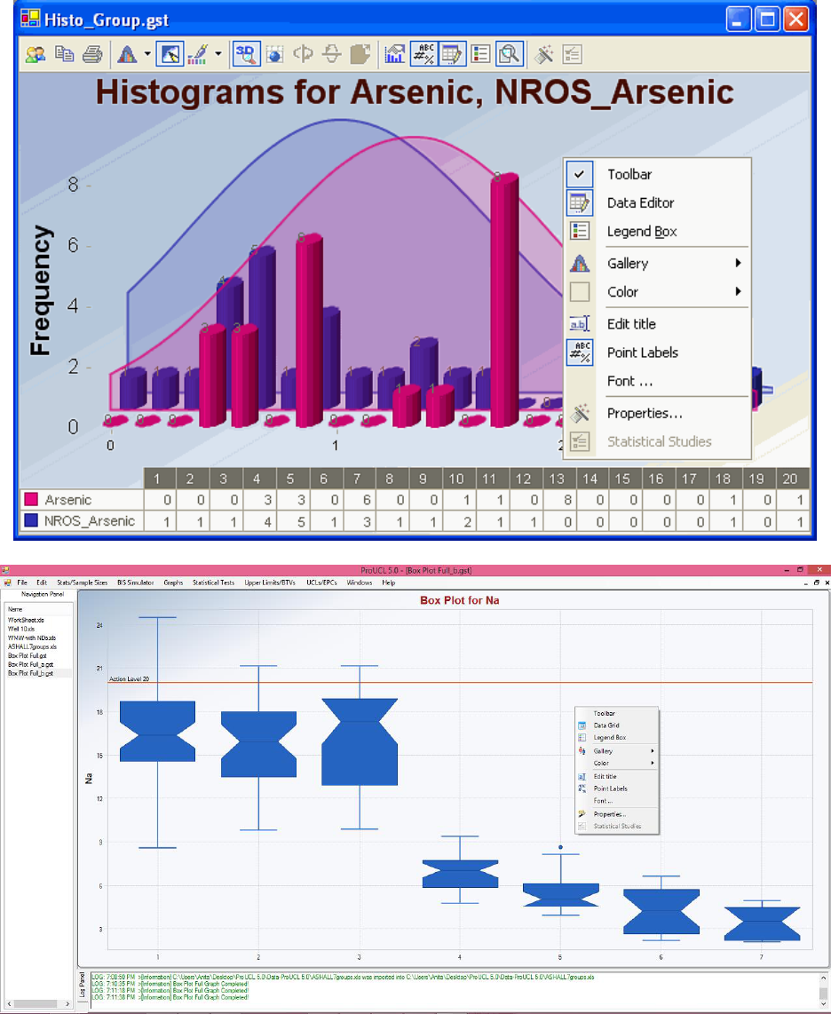
87

88
Chapter 3
Select Variables Screen
3.1 Select Variables Screen
The Select Variable screen is associated with all modules of ProUCL.
Variables need to be selected to perform statistical analyses.
When the user clicks on a drop-down menu for a statistical procedure (e.g., UCLs/EPCs), the
following window will appear.
The Options button is available in certain menus. The use of this option leads to another pop-
up window such as shown below. This window provides the options associated with the
selected statistical method (e.g., BTVs, OLS Regression).
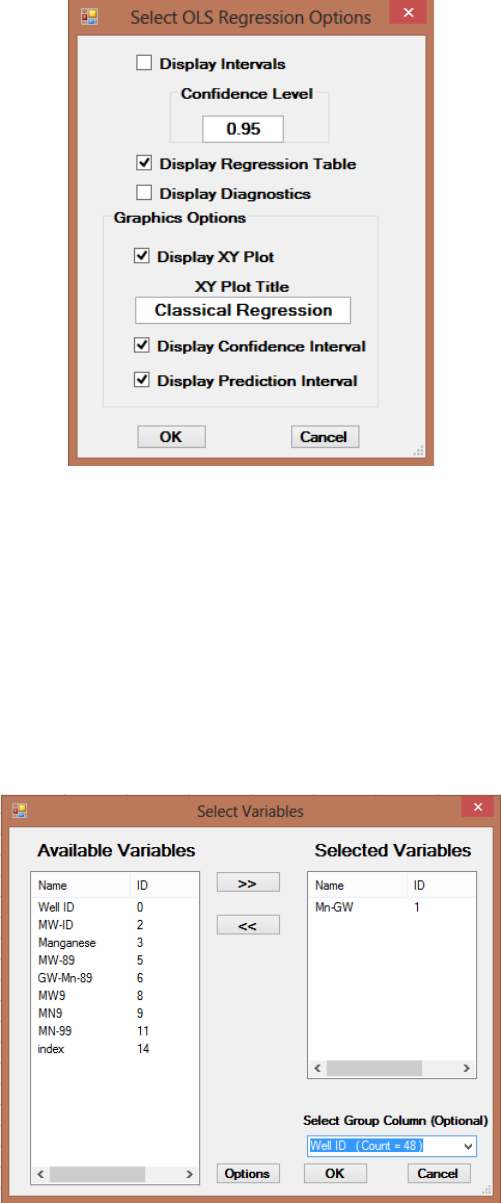
89
ProUCL can process multiple variables simultaneously. ProUCL software can generate
graphs, and compute UCLs, and background statistics simultaneously for all selected
variables shown in the right panel of the screen shot displayed on the previous page.
If the user wants to perform statistical analysis on a variable (e.g., manganese) by a Group
variable, click the arrow below the Select Group Column (Optional) to get a drop-down list
of available variables from which to select an appropriate group variable. For example, a
group variable (e.g., Well ID) can have alphanumeric values such as MW8, MW9, and MW1.
Thus in this example, the group variable name, Well ID, takes 3 values: MW1, MW8, and
MW9. The selected statistical method (e.g., GOF test) performs computations on data sets for
all the groups associated with the selected group variable (e.g., Well ID)
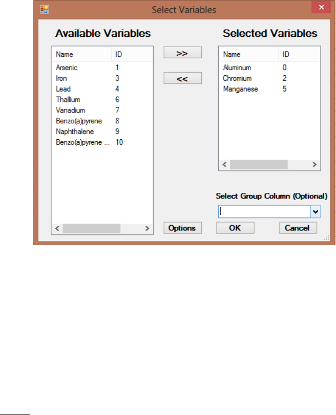
90
The Group variable is useful when data from two or more samples need to be compared.
Any variable can be a group variable. However, for meaningful results, only a variable,
that really represents a group variable (categories) should be selected as a group variable.
The number of observations in the group variable and the number observations in the
selected variables (to be used in a statistical procedure) should be the same. In the
example below, the variable “Mercury” is not selected because the number of
observations for Mercury is 30; in other words mercury values have not been grouped.
The group variable and each of the selected variables have 20 data values.
As mentioned earlier, one should not assign any missing value such as a “Blank” for the
group variable. If there is a missing value (represented by blanks, strings or 1E31) for a
group variable, ProUCL will treat those missing values as a new group. As such, data
values corresponding to the missing Group will be assigned to a new group.
The Group Option is a useful tool for performing statistical tests and methods (including
graphical displays) separately for each of the group (samples from different populations)
that may be present in a data set. For example, the same data set may consist of samples
from multiple populations. The graphical displays (e.g., box plots, Q-Q plots) and
statistics of interest can be computed separately for each group by using this option.
Notes: Once again, care should be taken to avoid misrepresentation and improper use of
group variables. Do not assign any form of a missing value for the group variable.
3.1.1 Graphs by Groups
The following options are available to generate graphs by groups.
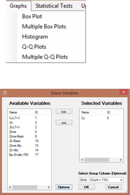
91
Individual or multiple graphs (Q-Q plots, box plots, and histograms) can be displayed on
a graph by selecting the Group Column (Optional) option shown as follows.
An individual graph for each group (specified by the selected group variable) is produced
by selecting the Individual Graph option; and multiple graphs (e.g., side-by-side box
plots, multiple Q-Q plots on the same graph) are produced by selecting the Group
Graph option as shown below. Using the Group Graph option, multiple graphs are
displayed for all sub-groups included in the Group variable. This option is used when
data are given in the same column and are classified by a group variable.

92
Multiple graphs for selected variables are produced by selecting options: Multiple Box
Plots or Multiple Q-Q Plots. Using the Group Graph option, multiple graphs for all
selected variables are shown on the same graphical display. This option is useful when
data (e.g., site lead and background lead) to be compared are given in different columns.
Notes: It should be noted that it is the users’ responsibility to provide an adequate amount of detected data
to perform the group operations. For example, if the user desires to produce a graphical Q-Q plot (using
only detected data) with regression lines displayed, then there should be at least two detected points (to
compute slope, intercept, and sd) in the data set. Similarly, if graphs are desired for each group specified
by a Group ID variable, there should be at least two detected observations in each group specified by the
Group ID variable. ProUCL displays a warning message (in orange) in the lower Log Panel of the
ProUCL screen when not enough data are available to perform a statistical or graphical operation.
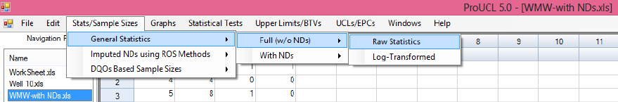
93
Chapter 4
General Statistics
The General Statistics option is available under the Stats/Sample Sizes module of ProUCL 5.0. This
option is used to compute general statistics including simple summary statistics (e.g., mean, standard
deviation) for all selected variables. In addition to simple summary statistics, several other statistics are
computed for full uncensored data sets (Full w/o NDs), and for data sets with nondetect (with NDs)
observations (e.g., estimates based upon the KM method). Two Menu options: Full w/o NDs and With
NDs are available.
Full (w/o NDs): This option computes general statistics for all selected variables.
With NDs: This option computes general statistics including the KM method based mean
and standard deviations for all selected variables with ND observations.
Each menu option (Full (w/o NDs) and With NDs) has two sub-menu options:
Raw Statistics
Log-Transformed
When computing general statistics for raw data, a message will be displayed for each variable that
contains non-numeric values. The General Statistics option computes log-transformed (natural log)
statistics only if all of the data values for the selected variable(s) are positive real numbers. A message
will be displayed if non-numeric characters, zero, or negative values are found in the column
corresponding to a selected variable.
4.1 General Statistics for Full Data Sets without NDs
1. Click General Statistics ► Full (w/o NDs)
2. Select either Log-Transformed or Raw Statistics option.
3. The Select Variables screen (see Chapter 3) will appear.
Select one or more variables from the Select Variables screen.
If statistics are to be computed by a Group variable, then select a group variable by
clicking the arrow below the Select Group Column (Optional) button. This will result
in drop-down list of available variables, and select a proper group variable.
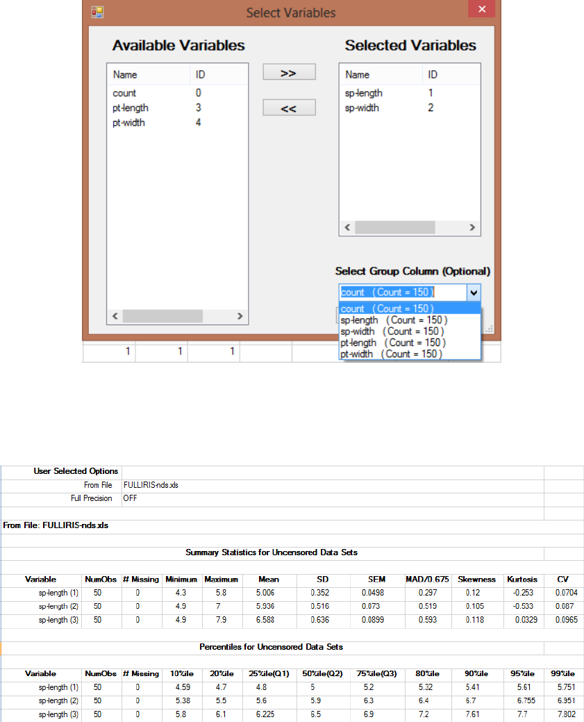
94
Click on the OK button to continue or on the Cancel button to cancel the General
Statistics option.
Raw Statistics
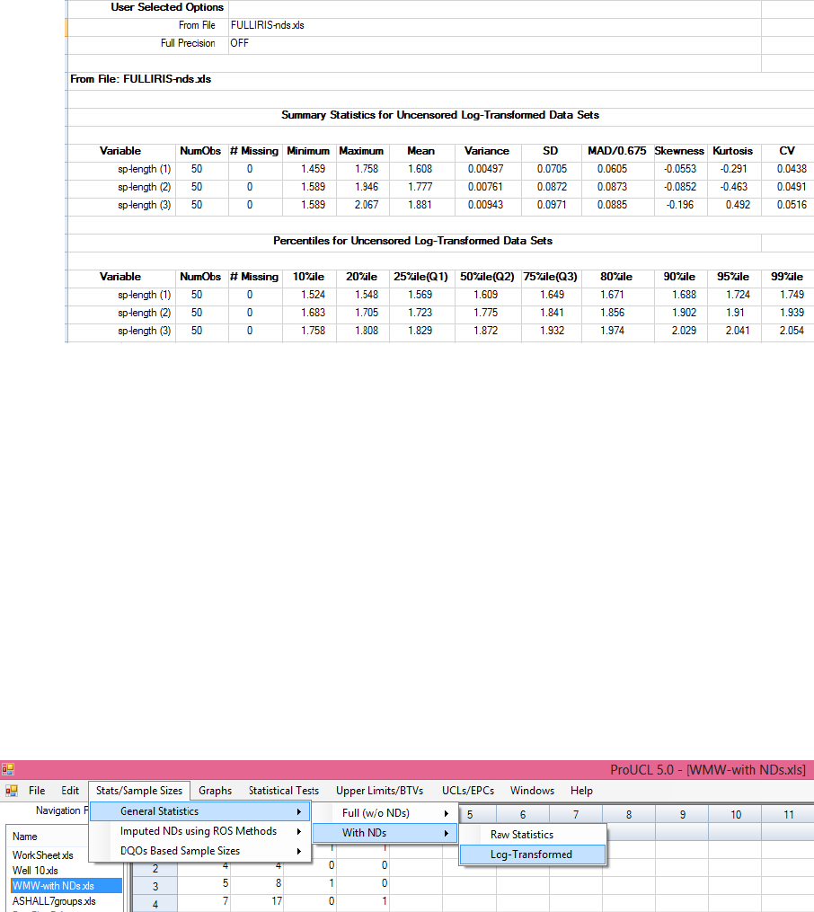
95
Log-Transformed Statistics
4. The General Statistics screen (and all other output screens generated by other modules) shown
above can be saved as an Excel 2003 (.xls) or 2007 (.xlsx) file. Click Save from the file menu.
5. On the output screen shown above, most of the statistics are self explanatory and described in the
ProUCL Technical Guide (EPA 2013, 2015). A couple of simple robust statistics (Hoaglin,
Mosteller, and Tukey 1983) included in the above output are described as follows.
MAD = Median absolute deviation
MAD/0.675 = Robust and resistant (to outliers) estimate of variability, population
standard deviation,
4.2 General Statistics with NDs
1. As above, Click General Statistics ► With NDs
2. Select either Log-Transformed or Raw Statistics option.
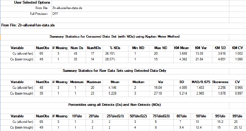
96
3. The Select Variables screen (Chapter 3) will appear.
Select variable(s) from the list of variables.
Only those variables that have ND values will be shown. The user should make sure that the
variables with NDs are defined properly including the column showing the detection status of
the various observations.
If statistics are to be computed by a Group variable, then select a group variable by clicking
the arrow below the Select Group Column (Optional) button. This will result in a drop-
down list of available variables. Select a proper group variable.
Click on the OK button to continue or on the Cancel button to cancel the summary statistics
operations.
Raw Statistics – Data Set with NDs
The Summary Statistics screen shown above can be saved as an Excel 2003 or 2007 file.
Click Save from the file menu.
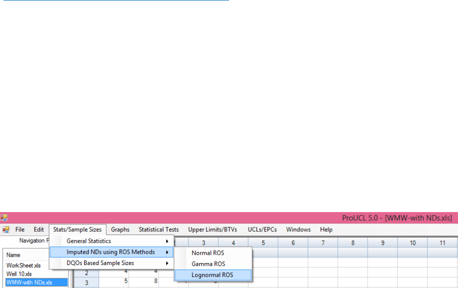
97
Chapter 5
Imputing Nondetects Using ROS Methods
The imputing of NDs using regression on order statistics (ROS) methods option is available under the
Stats/Sample Sizes module of ProUCL 5.1. This option is provided for advanced users who want to use
the detected and imputed NDs data for exploratory and data mining purposes on multivariate data sets.
For exploratory methods, such as principal component analysis (PCA), cluster, and discriminant analysis
to gain additional insight into potential structures and patterns present in a multivariate (more than one
variable) data set, one may want to use imputed values in graphical displays (line graphs, scatter plots,
boxplots etc.) and in the analyses. To derive conclusions based upon multivariate data sets with
nondetects, the developers suggest the use of the KM method based covariance or correlation matrix to
perform PCA and regression analysis. These methods are beyond the scope of the ProUCL software
which deals only with univariate methods. The details of computing an Orthogonalized Kettenring and
Gnanadesikan (OKG) positive definite KM matrix can be found in Maronna, Martin, and Yohai (2006)
and in Scout 2008 Version 1.0 guidance documents (2009) which can be downloaded from the EPA Site
(http://archive.epa.gov/esd/archive-scout/web/html/). One may not use ROS imputed data to perform
parametric statistical tests such as t-test and ANOVA test without further investigation. These issues
require further research to evaluate decision errors associated with conclusions derived using such
methods.
The ROS methods can be used to impute ND observations using a normal, lognormal, or gamma model.
ProUCL has three ROS estimation methods that can be used to impute ND observations. The use of this
option generates additional columns consisting of all imputed NDs and detected observations. These
columns are appended to the existing open spreadsheet file. The user should save the updated file if they
want to use the imputed data for their other application(s) such as PCA or discriminant analysis. It is not
easy to perform multivariate statistical methods on data sets with NDs. The availability of imputed NDs
in a data file helps the advanced users who want to use exploratory methods on data sets with ND
observations. Like other statistical methods in ProUCL, NDs can also be imputed by a group variable.
One can impute NDs using the following steps.
1. Click Imputed NDs using ROS Methods ► Lognormal ROS
2. The Select Variables screen (Chapter 3) will appear.
Select one or more variable(s) from the Select Variables screen; NDs can be imputed
using a group variable as shown in the following screen shot.
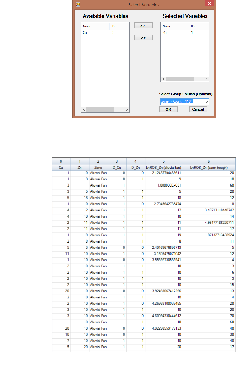
98
Click on the OK button to continue or on the Cancel button to cancel the option.
Output Screen for ROS Est. NDs (Lognormal ROS) Option
Notes: For grouped data, ProUCL generates a separate column for each group in the data set as shown in
the above table. Columns with a similar naming convention are generated for each selected variable and
distribution using the ROS option.
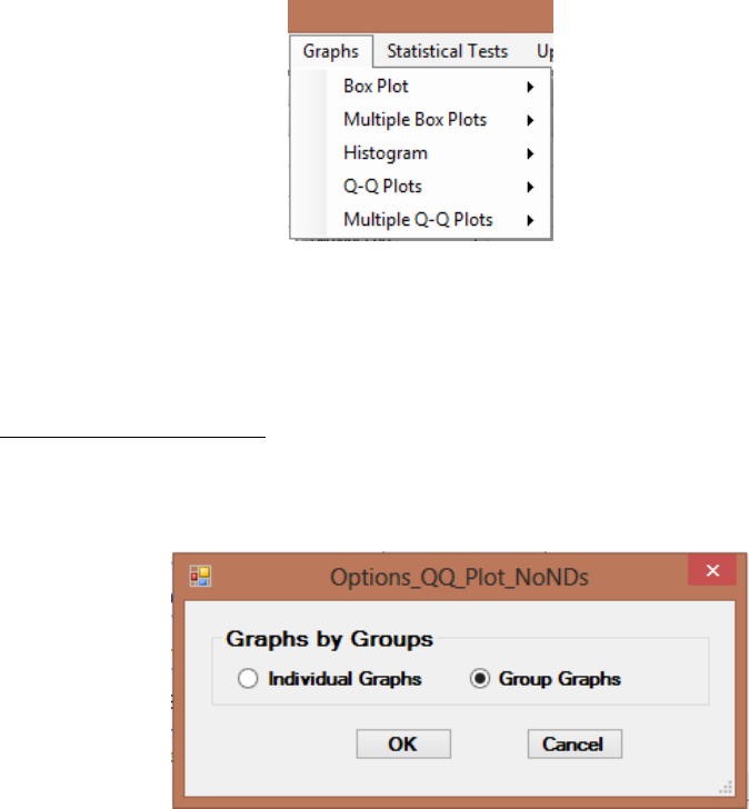
99
Chapter 6
Graphical Methods (Graph)
The graphical methods described here are used as exploratory tools to get some idea about data
distributions (e.g., skewed, symmetric), potential outliers and/or multiple populations present in a data
set. The following graphical methods are available under the Graphs option of ProUCL 5.1
All graphical displays listed above can be generated using uncensored full data sets (Full w/o
NDs) as well as left-censored data sets with nondetect (With NDs) observations. On box plot
graphs for data sets with NDs, a horizontal line is also displayed at the highest RL/DL
associated with ND observations.
Q-Q Plots and Histograms: Q-Q plots and histograms can be generated individually as well as
by using a Group variable. Graphs generated using the Group Graphs option shown below is
useful when data for selected variable(s) are given in the same column (stacked data)
categorized by a Group ID.
For data sets with NDs, three options described below are available to draw Q-Q plots and
histograms. Specifically, these graphs are displayed only for detected values, or with NDs
replaced by 1/2DL values, or with NDs replaced by the respective DLs. The statistics
displayed on a Q-Q plot (mean, sd, slope, intercept) are computed according to the selected
method. On Q-Q plots, ND values are displayed using a different symbol. The exploratory Q-
Q plots described here do not require any placeholders for NDs. These graphs are used only
to determine the distribution of detected values and to identify potential outliers and/or
multiple populations present in a data set. On histograms, the user can change the number of
bins (more bins, less bins) used to generate histograms.
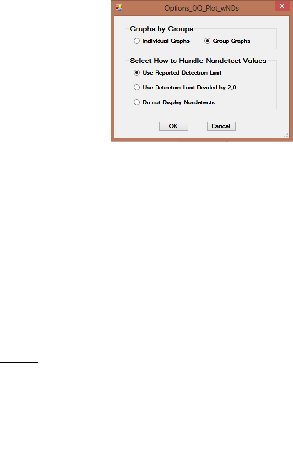
100
Do not Display Nondetects: Selection of this option excludes all NDs from a graphical
method (Q-Q plots and histograms) and plots only detected values. The statistics shown on
Q-Q plots are computed only using the detected data.
Use Reported Detection Limit: Selection of this option treats DLs/RLs as detected values
associated with the ND values. The graphs are generated using the numerical values of
detection limits and statistics displayed on Q-Q plots are computed accordingly.
Use Detection Limit Divided by 2.0: Selection of this option replaces the DLs with their half
values. All Q-Q plots and histograms are generated using the half detection limits and
detected values. The statistics displayed on Q-Q plots are computed accordingly.
For data sets in different columns, one can use the Multiple Q-Q Plots option. By default,
this option will display multiple Q-Q plots for all selected variables on the same graph. One
can also generate multiple Q-Q plots by using a group variable.
Box Plot: Like Q-Q plots, box plots can also be generated by a Group variable. This option is
useful when all data are listed in the same column (stacked data) categorized by a Group ID
variable. On box plots with NDs, a horizontal line is displayed at the highest detection limit
level. ProUCL 5.1 constructs a box plot using all detected and nondetected (using associated
DL values) values. A horizontal line is displayed at the highest detection limit. Box Plots are
generated using ChartFx, a software used in the development of ProUCL 5.1.
Multiple Box Plots: For data in different columns, one can use the Multiple Box Plots option
to display multiple box plots for all selected variables on the same graph. One can also
generate multiple box plots by using a group variable.
Box Plots have an optional feature, which can be used to draw up to four (4) horizontal lines
at pre-established screening levels or at statistical limits (e.g., upper limits) computed using a
background data set. This option can be used when box plots are generated using onsite data
and one may be interested in comparing onsite data with background threshold values and/or
pre-established screening levels. This type of box plot represents a visual comparison of site
data with background threshold values and/or other action levels. Up to four (4) values can be
displayed on a box plot as shown below. If the user inputs a value in the value column, the
check box in that row will get activated. For example, the user may want to display horizontal
lines at a background UTL95-95 or some pre-established action level(s) on box plots
generated using AOCs data.
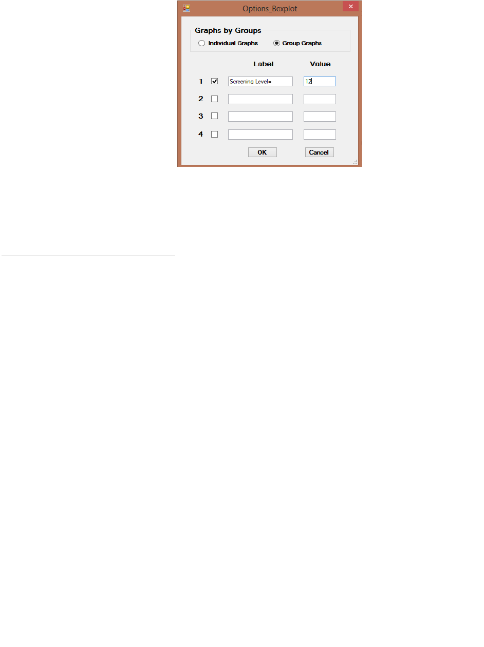
101
6.1 Box Plot
A brief description of the method used to generate Tukey's box plot (also known as box and whisker plot)
is described first.
Box Plot (Box and Whiskers Plot): A box plot (box and whiskers plot) represents a convenient
exploratory tool and provides a quick five-point summary of a data set. In statistical literature, one can
find several ways to generate box plots. The practitioners may have their own preferences to use one
method over the other. Box plots are well documented in the statistical literature and a description of box
plots can be easily obtained by surfing the net. Therefore, a detailed description about the generation of
box plots is not provided in ProUCL guidance documents.
All box plot methods including the one in ProUCL represent five-point summary graphs including: the
lowest and the highest data values, median (50
th
percentile=second quartile, Q2), 25
th
percentile (lower
quartile, Q1), and 75
th
percentile (upper quartile, Q3). A box and whisker plot also provides information
about the degree of dispersion (interquartile range (IQR) = Q3-Q1=length/height of the box in a box plot),
the degree of skewness (suggested by the length of the whiskers) and unusual data values known as
outliers. Specifically, ProUCL (and various other software packages) use the following to generate a box
and whisker plot.
Q1= 25
th
percentile, Q2= 50
th
(median), and Q3 = 75
th
percentile
Interquartile range= IQR = Q3-Q1 (the height of the box in a box plot)
Lower whisker starts at Q1 and the upper whisker starts at Q3.
Lower whisker extends up to the lowest observation or (Q1 - 1.5 * IQR) whichever is higher
Upper whisker extends up to the highest observation or (Q3 + 1.5 * IQR) whichever is lower
Horizontal bars (also known as fences) are drawn at the end of whiskers
Observations lying outside the fences (above the upper bar and below the lower bar) represent
potential outliers
ProUCL uses a couple of development tools such as FarPoint spread (for Excel type input and output
operations) and ChartFx (for graphical displays). ProUCL generates box plots using the built-in box plot
feature in ChartFx. The programmer has no control over computing the statistics (e.g., Q1, Q2, Q3, IQR)
using ChartFx. Boxplots generated by ProUCL can slightly differ from box plots generated by other
programs (e.g., Excel). However, for all practical and exploratory purposes, box plots in ProUCL are
equally good (if not better) than those available in the various commercial software packages for
exploring data distribution (skewed or symmetric), identifying outliers, and comparing multiple groups
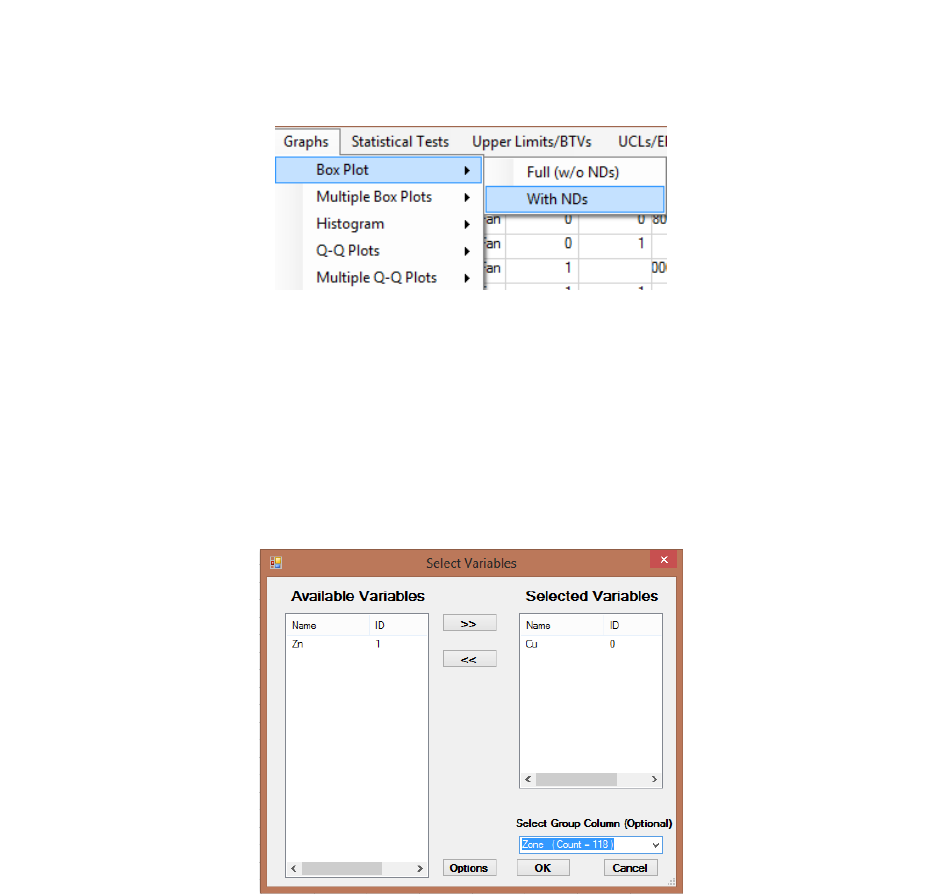
102
(main objectives of box plots in ProUCL). More details about Box Plots can be found in Section 1.16 of
Chapter 1 of this document.
1. Click Graphs ► Box Plot
2. The Select Variables screen (Chapter 3) will appear.
Select one or more variable(s) from the Select Variables screen.
If graphs are to be produced by using a Group variable, select a group variable by
clicking the arrow below the Select Group Column (Optional) button. This will result
in a drop-down list of available variables. The user should select an appropriate variable
representing a group variable as shown below.
The default option for Graph by Groups is Group Graphs. This option produces side-by-
side box plots for all groups included in the selected Group ID Column (e.g., Zone here). The
Group Graphs option is used when multiple graphs categorized by a group variable need to
be produced on the same graph. The Individual Graphs option generates individual graphs
for each selected variable or one box plot for each group for the variable categorized by a
Group ID column (variable).
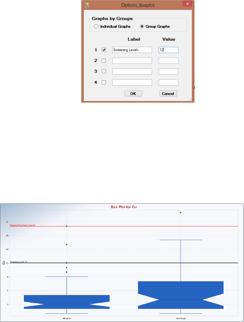
103
While generating box plots, one can display horizontal lines at specified screening levels
or a BTV estimate (e.g., UTL95-95) computed using a background data set. For data sets
with NDs, a horizontal line is also displayed at the largest reported DL associated with a
ND value. The use of this option may provide information about the analytical methods
used to analyze field samples.
Click on the OK button to continue or on the Cancel button to cancel the Box Plot (or
other selected graphical) option.
Box Plot Output Screen (Group Graph)
Selected options: Label (Screening Level), Value (12)
Making Changes in Graphs using Toolbar
One can use the toolbar to make changes in a graph generated by ProUCL. The toolbar can be activated
by right clicking the mouse on your graph. The context menu on the box plot shown below appears. By
using the context menu, one can change color, title, font size, legend box and label points. For example,
one can edit the title by clicking title in the context menu. These are typical windows operations which
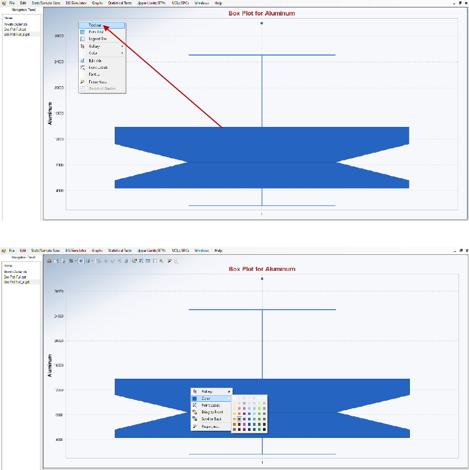
104
can also be used in ProUCL. However, it should be pointed out that options which affect the computation
of statistics displayed on a graph are not wired and can yield incorrect results. For example, changing
scales along the x-axis or y-axis (e.g., to log scale) will not automatically displayed statistics in the
changed log- scale. The resulting graph using options that affect computed statistics will be incorrect and
should be avoided. These operations are illustrated by several screen captures displayed as follows.
Activating the toolbar shown above.
Changing color of the graph shown in the above graph.
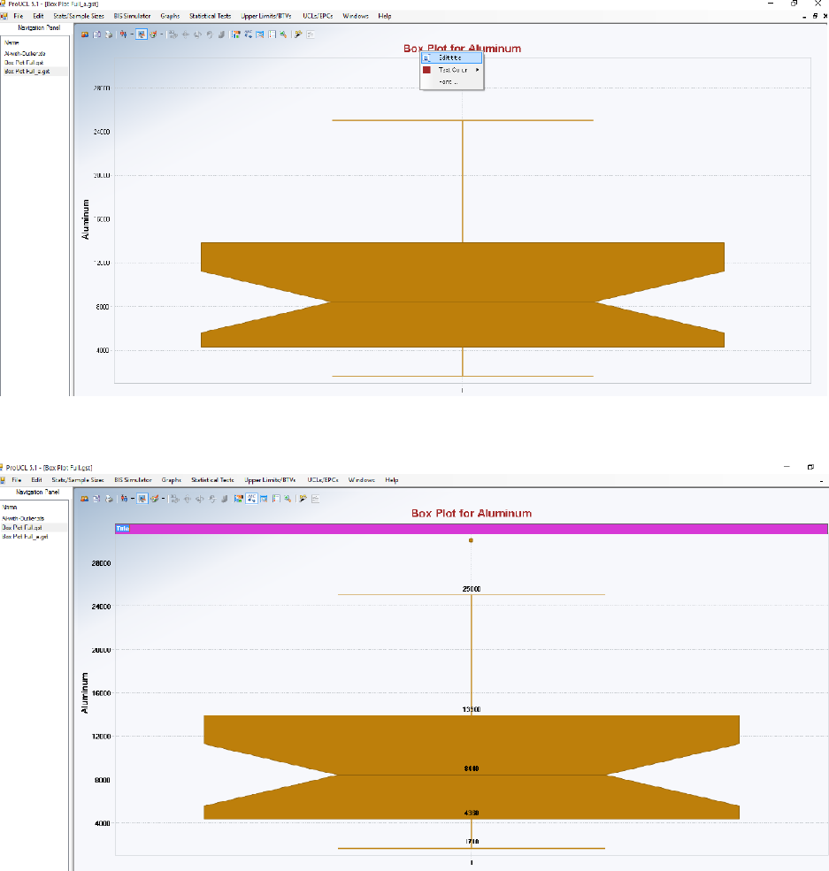
105
Changing title of the graph.
Edit the title of the graph.
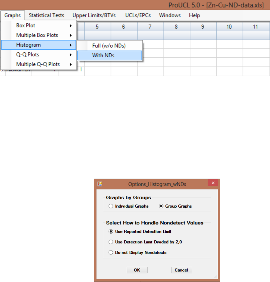
106
6.2 Histogram
1. Click Graphs ► Histogram
2. The Select Variables screen (Chapter 3) will appear.
Select one or more variable(s) from the Select Variables screen.
If graphs have to be produced by using a Group variable, then select a group variable by
clicking the arrow below the Select Group Column (Optional) button. This will result
in a drop-down list of available variables. The user should select an appropriate variable
representing a group variable as shown below.
When the option button is clicked for data sets with NDs, the following window will be
shown. By default, histograms are generating using the RLs for NDs.
The default selection for histograms (and for all other graphs) by a group variable is
Group Graphs. This option produces multiple histograms on the same graph. If
histograms are needed to be displayed individually, the user should check the radio
button next to Individual Graphs.
Click on the OK button to continue or on the Cancel button to cancel the histogram (or
other selected graphical) option.
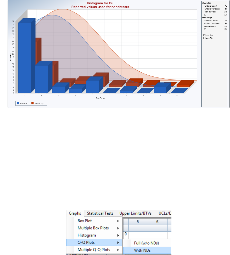
107
Histogram Output Screen
Selected options: Group Graphs
Notes: ProUCL does not perform any GOF tests when generating histograms. Histograms are generated
using the development software ChartFx and not many options are available to alter the histograms. The
labeling along the x-axis is done by the development software and it is less than perfect. However, if one
hovers the mouse on a bar, relevant statistics (e.g., begin point, midpint and end point) about the bar will
appear on the screen. The Histogram option automatically generates a normal probability density
function (pdf) curve irrespective of the data distribution. At this time, ProUCL 5.1 does not display a pdf
curve for any other distribution (e.g., gamma) on a historgram. The user can increase or decrease the
number of bins to be used in a histogram.
6.3 Q-Q Plots
1. Click Graphs ► Q-Q Plots. When that option button is clicked, the following window will
be shown.
2. Q-Q Plots can be generated for data sets With NDs and without NDs [Full (w/o NDs)].
Select either Full (w/o NDs) or With NDs option.
The Select Variables screen (Chapter 3) will appear.
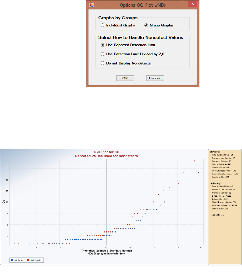
108
Select one or more variable(s) from the Select Variables screen.
If graphs have to be produced by using a group variable, then select a group variable by
clicking the arrow below the Select Group Column (Optional) button. This will result in a
drop-down list of available variables. The user should select and click on an appropriate
variable representing a group variable as shown below.
Click on the OK button to continue or on the Cancel button to cancel the selected Q-Q plots
option. The following options screen appears providing choices on how to treat NDs. The
default option is to use the reported values for all NDs.
Click on the OK button to continue or on the Cancel button to cancel the selected Q-Q plots
option. The following Q-Q plot appears when used on the copper concentrations of two
zones: Alluvial Fan and Basin Trough.
Output Screen for Q-Q plots (With NDs)
Selected options: Group Graph, No Best Fit Line
Note: The font size of ND values is smaller than that of the detected values.
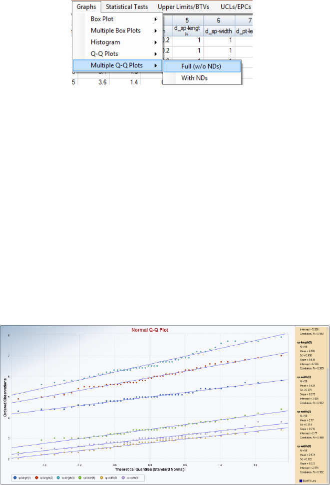
109
6.4 Multiple Q-Q Plots
6.4.1 Multiple Q-Q plots (Uncensored data sets)
1. Click Graphs ► Multiple Q-Q Plots
2. Multiple Q-Q Plots can be generated for data sets With NDs and without NDs [Full (w/o
NDs)].
When that Option button is clicked, the following window will be shown.
Select either Full (w/o NDs) or With NDs.
The Select Variables Screen (Chapter 3) will appear.
Select one or more variable(s) from the Select Variables screen.
If graphs have to be produced by using a Group variable, then select a group variable by
clicking the arrow below the Select Group Column (Optional) button. This will result in a
drop-down list of available variables. The user should select and click on an appropriate
variable representing a group variable as shown below.
Click OK to continue or Cancel button to cancel the selected Multiple Q-Q Plots option.
Example 6-1: The following graph is generated by using Fisher's (1936) data set for 3 Iris species.
Output Screen for Multiple Q-Q Plots (Full w/o NDs)
Selected Options: Group Graph, Best Fit Line
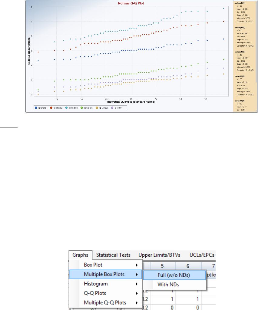
110
If the user does not want the regression lines shown above, click on the Best Fit Line and all regression
lines will disappear as shown below.
Notes: For Q-Q plots and Multiple Q-Q plots option, for both “Full” as well as for data sets “With NDs,”
the values along the horizontal axis represent quantiles of a standardized normal distribution (Normal
distribution with mean=0 and standard deviation=1). Quantiles for other distributions (e.g., Gamma
distribution) are used when using the Goodness-of-Fit (GOF, G.O.F.) test option.
6.5 Multiple Box Plots
6.5.1 Multiple Box plots (Uncensored data sets)
1. Click Graphs ► Multiple Box Plots
2. Multiple Q-Q Plots can be generated for data sets With NDs and without NDs [Full (w/o
NDs)].
When the option button is clicked, the following window will be shown.
Select either Full (w/o NDs) or With NDs.
The Select Variables screen (Chapter 3) will appear.
Select one or more variable(s) from the Select Variables screen.
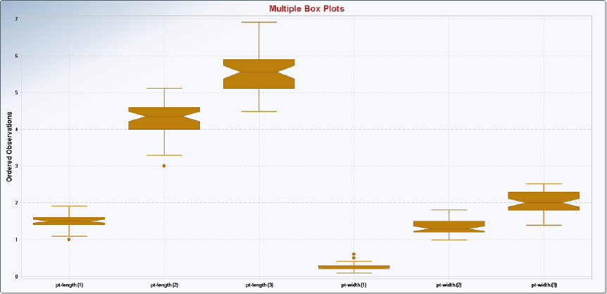
111
If graphs have to be produced by using a Group variable, then select a group variable by
clicking the arrow below the Select Group Column (Optional) button. This will result in a
drop-down list of available variables. The user should select and click on an appropriate
variable representing a group variable as shown below.
Click on the OK button to continue or on the Cancel button to cancel the selected Multiple
Box Plots options. The following graph is generated by using the above options.
Example 6-1 (continued): The following graph is generated by using the above options on Fisher's
(1936) Iris data set collected from 3 species of Iris flower.
Output Screen for Multiple Box Plots (Full w/o NDs)
Selected options: Group Graph

112
Chapter 7
Classical Outlier Tests
Outliers are inevitable in data sets originating from environmental applications. In addition to informal
graphical displays (e.g., Q-Q plots and box plots) and classical outlier tests (Dixon test, Rosner test), there
exist several robust outlier identification methods (e.g., Biweight, Huber, PROP, MCD) for identifying
any number of multiple outliers present in data sets of various sizes (Scout 2008; EPA 2009). It is well
known that the classical outlier tests: Dixon test and Rosner test suffer from masking (e.g., extreme
outliers may mask intermediate outliers) effects. The use of robust outlier identification procedures is
recommended for identifying multiple outliers, especially when dealing with multivariate (having
multiple constituents) data sets. However, those preferred and more efficient robust outlier identification
methods are beyond the scope of ProUCL 5.1. Several robust outlier identification methods (e.g., based
upon Biweight, Huber, and PROP influence functions, Singh and Nocerino 1995) are available in the
Scout 2008 v1.0 software package (EPA, 2009).
The two classical outlier tests: Dixon and Rosner tests (EPA 2006a; Gilbert 1987) are available in
ProUCL 4.0 and higher versions of the ProUCL software. These tests can be used on data sets with and
without ND observations. These tests require the assumption of normality of the data set without the
outliers; as data sets consisting of outliers seldom follow a normal distribution. It should be noted that in
environmental applications, one of the objectives is to identify high outlying observations that might be
present in the right tail of a data distribution, as those observations often represent contaminated locations
requiring further investigations. Therefore, for data sets with NDs, two options are available in ProUCL to
deal with data sets with outliers. These options are: 1) exclude NDs and 2) replace NDs by DL/2 values.
These options are used only to identify outliers and not to compute any estimates and limits used in
decision-making processes. To compute the various statistics of interest, ProUCL uses rigorous statistical
methods suited for left-censored data sets with multiple DLs.
It is suggested that the outlier identification procedures be supplemented with graphical displays such as
normal Q-Q plots and box plots. On a normal Q-Q plot, observations that are well-separated from the
bulk of the data typically represent potential outliers needing further investigation. Also, significant and
obvious jumps and breaks in a normal Q-Q plot can be indications of the presence of more than one
population and/or data gaps due to lack of enough data points (data sets of smaller sizes). Data sets of
large sizes (e.g., >100) exhibiting such behavior on Q-Q plots may need to be partitioned out into
component sub-populations before estimating EPCs or BTVs.
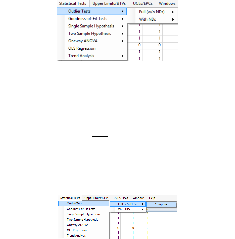
113
Outlier tests in ProUCL 5.1 are available under the Statistical Tests module.
Dixon's Outlier Test (Extreme Value Test): Dixon's test is used to identify statistical outliers when the
sample size is ≤ 25. This test identifies outliers or extreme values in the left tail (Case 2) and also in the
right tail (Case 1) of a data distribution. In environmental data sets, outliers found in the right tail,
potentially representing impacted locations, are of interest. The Dixon test assumes that the data without
the suspected outlier (s) are normally distributed. If the user wants to perform a normality test on the data
set, he should first remove the outliers before performing the normality test. This test tends to suffer from
masking in the presence of multiple outliers. This means that if more than one outlier (in either tail) is
suspected, this test may fail to identify all of the outliers.
Rosner Outlier Test: This test can be used to identify up to 10 outliers in data sets of sizes 25 and higher.
This test also assumes that the data set without the suspected outliers is normally distributed. Like the
Dixon test, if the user wants to perform a normality test on the data set, he should first remove the outliers
(which are not known in advance) before performing the normality test. The detailed discussion of these
two tests is given in the associated ProUCL Technical Guide. A couple of examples illustrating the
identification of outliers in data sets with NDs are described in the following sections.
7.1 Outlier Test for Full Data Set
1. Click Outlier Tests ► Full (w/o NDs) ►Compute
2. The Select Variables screen (Chapter 3) will appear.
Select one or more variable(s) from the Select Variables screen.
If outlier test needs to be performed by using a Group variable, then select a group variable
by clicking the arrow below the Select Group Column (Optional) button. This will result in
a drop-down list of available variables. The user should select and click on an appropriate
variable representing a group variable.
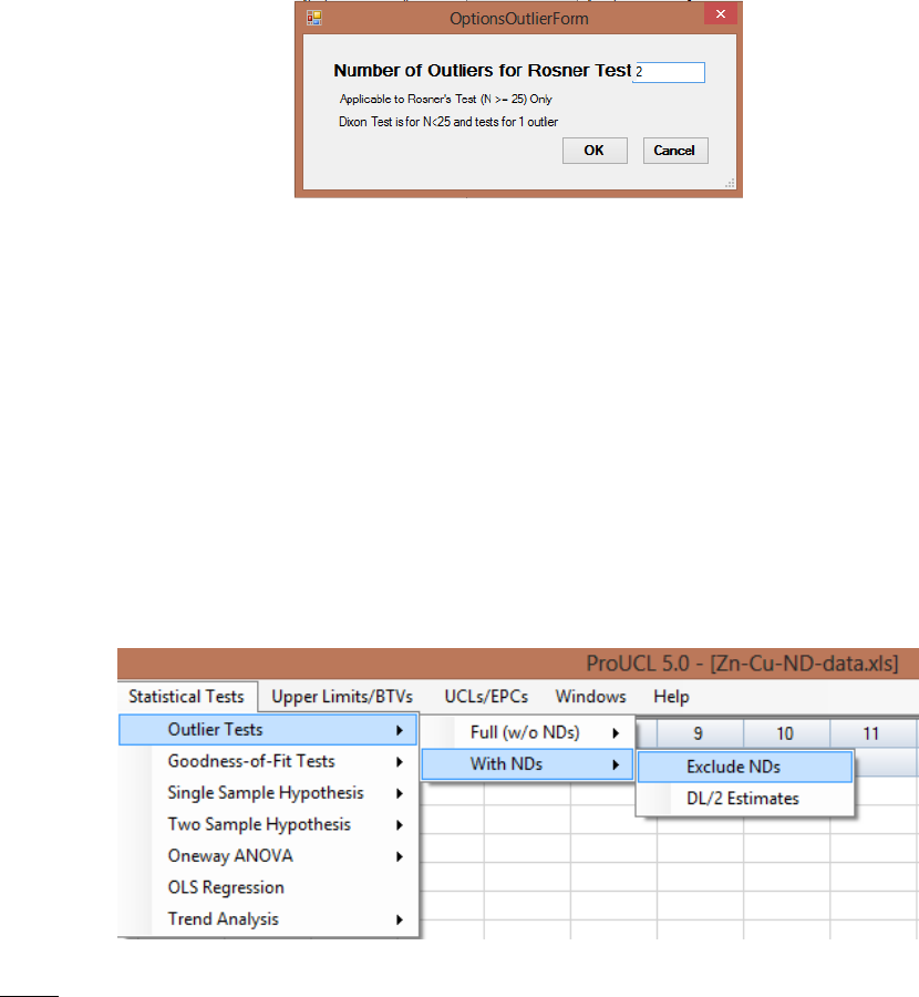
114
If at least one of the selected variables (or group) has 25 or more observations, then click the
option button for the Rosner Test. ProUCL automatically performs the Dixon test for data
sets of sizes ≤ 25.
The default option for the number of suspected outliers is 1. To use the Rosner test, the user
has to obtain an initial guess about the number of suspected outliers that may be present in the
data set. This can be done by using graphical displays such as a Q-Q plot. On a Q-Q plot,
higher observations that are well separated from the rest of the data may be considered as
potential or suspected outliers.
Click on the OK button to continue or on the Cancel button to cancel the Outlier Test.
7.2 Outlier Test for Data Sets with NDs
Two options: exclude NDs; or replace NDs by their respective DL/2 are available in ProUCL to perform
outlier tests on data sets with NDs.
1. Click Outlier Tests ► With NDs ► Exclude NDs
Note: The above screen shot was generated using ProUCL 5.0; the exactly similar screen is
generated using ProUCL 5.1 with the exception that in the title of the screen shot, ProUCL 5.0
will be replaced by ProUCL 5.1. Therefore, to save time, many intermediate screen shots used in
the ProUCL 5.0 User Guide have been used in this ProUCL 5.1 User Guide.
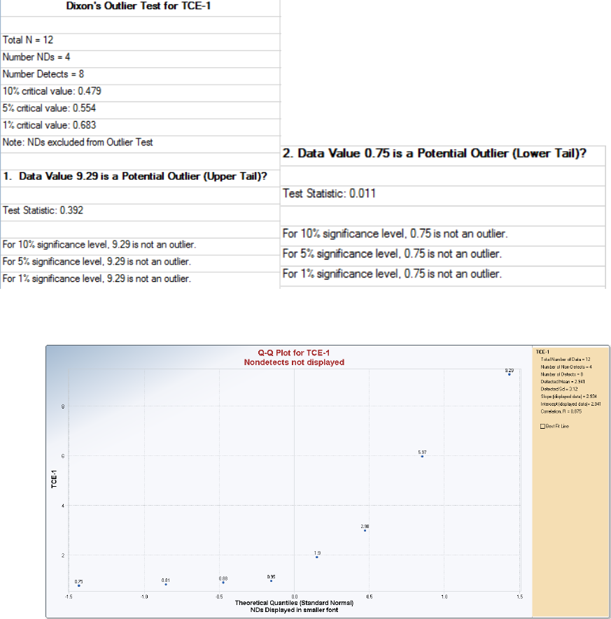
115
Output Screen for Dixon’s Outlier Test
Q-Q plot without Four Nondetect Observations are Shown as Follows
Example: Rosner’s Outlier Test by a Group Variable, Zone
Selected Options: Number of Suspected Outliers = 4
NDs excluded from the Rosner Test
Outlier test performed using the Select Group Column (Optional)

116
Output Screen for Rosner’s Outlier Test for Zinc in Zone: Alluvial Fan
Q-Q plot for Zinc Based upon Detected Data (Alluvial Fan)
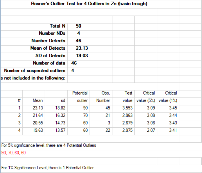
117
Output Screen for Rosner’s Outlier Test for Zinc in Zone: Basin Trough
118
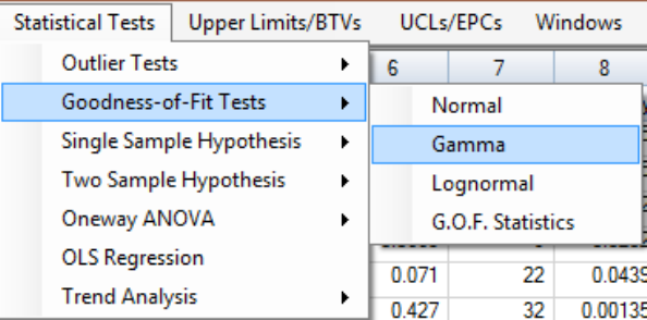
119
Chapter 8
Goodness-of-Fit (GOF) Tests for Uncensored and Left-Censored
Data Sets
GOF tests are available under the Statistical Test module of ProUCL 5.0/ProUCL 5.1. Throughout this
User Guide and in ProUCL software, “Full” represents uncensored data sets without ND observations.
The details and usage of the various GOF tests are described in the associated ProUCL Technical Guide.
In ProUCL 5.1, critical values associated with Lilliefors normality test are computed using a more
efficient algorithm as described in the associated ProUCL 5.1 Technical Guide. Therefore, tables and
graphs involving Lilliefors test have been re-generated using ProUCL 5.1.
8.1 Goodness-of-Fit Test in ProUCL
Several GOF tests for uncensored full (Full (w/o NDs)) and left-censored (With NDs) data sets are
available in the ProUCL software.
Full (w/o NDs)
o This option is used on uncensored full data sets without any ND observations. This
option can be used to determine GOF for normal, gamma, or lognormal distribution
of the variable(s) selected using the Select Variables option.
o Like all other methods in ProUCL, GOF tests can also be performed on variables
categorized by a Group ID variable.
o Based upon the hypothesized distribution (normal, gamma, lognormal), a Q-Q plot
displaying all statistics of interest including the derived conclusion is also generated.
o The G.O.F. Statistics option generates a detailed output log (Excel type spreadsheet)
showing all GOF test statistics (with derived conclusions) available in ProUCL. This
option helps a user to determine the distribution of a data set before generating a
GOF Q-Q plot for the hypothesized distribution. This option was included at the
request of some users in earlier versions of ProUCL.
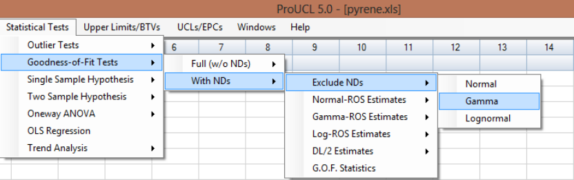
120
With NDs
o This option performs GOF tests on data sets consisting of both nondetected and
detected data values.
o Several sub-menu items shown below are available for this option.
1. Exclude NDs: tests for normal, gamma, or lognormal distribution of the selected
variable(s) using only the detected values.
2. ROS Estimates: tests for normal, gamma, or lognormal distribution of the selected
variable(s) using detected values and imputed nondetects.
o Three ROS methods for normal, lognormal (Log), and gamma distributions are
available. This option imputes the NDs based upon the specified distribution and
performs the specified GOF test on the data set consisting of detects and imputed
nondetects.
3. DL/2 Estimates: tests for normal, gamma, or lognormal distribution of the selected
variable(s) using the detected values and the ND values replaced by their respective
DL/2 values. This option is included for historical reasons and also for curious users.
ProUCL does not make any recommendations based upon this option.
4. G.O.F. Statistics: Like full uncensored data sets, this option generates an output log
of all GOF test statistics available in ProUCL for data sets with nondetects. The
conclusions about the data distributions for all selected variables are also displayed
on the generated output file (Excel-type spreadsheet).
Multiple variables: When multiple variables are selected from the Select Variables screen, one
can use one of the following two options:
o Use the Group Graphs option to produce multiple GOF Q-Q plots for all selected
variables in a single graph. This option may be used when a selected variable has data
coming from two or more groups or populations. The relevant statistics (e.g., slope,
intercept, correlation, test statistic and critical value) associated with the selected
variables are shown on the right panel of the GOF Q-Q plot. To capture all the graphs
and results shown on the window screen, it is preferable to print the graph using the

121
Landscape option. The user may also want to turn off the Navigation Panel and Log
Panel.
o The Individual Graphs option is used to generate individual GOF Q-Q plots for each of
the selected variables, one variable at a time (or for each group individually of the
selected variable categorized by a Group ID). This is the most commonly used option to
perform GOF tests for the selected variables.
GOF Q-Q plots for hypothesized distributions: ProUCL computes the relevant test statistic
and the associated critical value, and prints them on the associated Q-Q plot (called GOF Q-Q
plot). On a GOF Q-Q plot, the program informs the user if the data are gamma, normally, or
lognormally distributed.
o For all options described above, ProUCL generates GOF Q-Q plots based upon the
hypothesized distribution (normal, gamma, lognormal). All GOF Q-Q plots display several
statistics of interest including the derived conclusion.
o The linear pattern displayed by a GOF Q-Q plot suggests an approximate GOF for the
selected distribution. The program computes the intercept, slope, and the correlation
coefficient for the linear pattern displayed by the Q-Q plot. A high value of the correlation
coefficient (e.g., > 0.95) may be an indication of a good fit for that distribution; however, the
high correlation should exhibit a definite linear pattern in the Q-Q plot without breaks and
discontinuities.
o On a GOF Q-Q plot, observations that are well separated from the majority of the data
typically represent potential outliers needing further investigation.
o Significant and obvious jumps and breaks and curves in a Q-Q plot are indications of the
presence of more than one population. Data sets exhibiting such behavior of Q-Q plots may
require partitioning of the data set into component subsets (representing sub-populations
present in a mixture data set) before computing upper limits to estimate EPCs or BTVs. It is
recommended that both graphical and formal goodness-of-fit tests be used on the same data
set to determine the distribution of the data set under study.
Normality or Lognormality Tests: In addition to informal graphical normal and lognormal Q-Q
plots, a formal GOF test is also available to test the normality or lognormality of the data set.
o Lilliefors Test: a test typically used for samples of size larger than 50 (> 50). However, the
Lilliefors test (generalized Kolmogorov Smirnov [KS] test) is available for samples of all
sizes. There is no applicable upper limit for sample size for the Lilliefors test.
o Shapiro and Wilk (SW, S-W) Test: a test used for samples of size smaller than or equal to
2000 (<= 2000). In ProUCL 5.0, the SW test uses the exact SW critical values for samples of
size 50 or less. For samples of size, greater than 50, the SW test statistic is displayed along
with the p-value of the test (Royston 1982, 1982a).
Notes: As with other statistical tests, sometimes these two GOF tests might lead to different conclusions.
The user is advised to exercise caution when interpreting these test results. When one the GOF tests
passes the hypothesized distribution, ProUCL 5.0/ProUCL 5.1 determines that the data set follows an
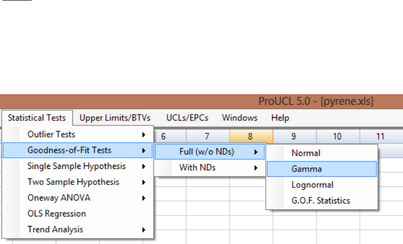
122
approximate hypothesized distribution. It should be pointed out that for data sets of smaller sizes (e.g.,
<50), when Lilliefors tests determines that the data set follows a normal (lognormal) distribution and
Shapiro-Wilk's test determines that the data set does not follow a normal (lognormal) distribution, the
user may not use the approximate normality (lognormality) conclusion derived using the Lilliefors test.
Under these situations, the user may determine the data distribution based upon the highest p-value
associated with GOF test statistics for other distributions or may determine that the data set does not
follow a discernible distribution.
GOF test for Gamma Distribution: In addition to the graphical gamma Q-Q plot, two formal
empirical distribution function (EDF) procedures are also available to test the gamma distribution
of a data set. These tests are the AD test and the KS test.
o It is noted that these two tests might lead to different conclusions. Therefore, the user should
exercise caution interpreting the results.
o These two tests may be used for samples of sizes in the range of 4 - 2500. Also, for these two
tests, the value (known or estimated) of the shape parameter, k (k hat) should lie in the
interval [0.01, 100.0]. Consult the associated ProUCL Technical Guide for a detailed
description of the gamma distribution and its parameters, including k. Extrapolation of critical
values beyond these sample sizes and values of k is not recommended.
Notes: Even though, the GOF Statistics option prints out all GOF test statistics for all selected
variables, it is suggested that the user should look at the graphical Q-Q plot displays to gain extra
insight (e.g., outliers, multiple population) into the data set.
8.2 Goodness-of-Fit Tests for Uncensored Full Data Sets
1. Click Goodness-of-Fit Tests ► Full (w/o NDs)
2. Select the distribution to be tested: Normal, Lognormal, or Gamma
To test for normality, click on Normal from the drop-down menu list.
To test for lognormality, click on Lognormal from the drop-down menu list.
To test for gamma distribution, click on Gamma from the drop-down menu list.

123
8.2.1 GOF Tests for Normal and Lognormal Distribution
1. Click Goodness-of-Fit Tests ► Full (w/o NDs) ► Normal or Lognormal
2. The Select Variables screen (Chapter 3) will appear.
Select one or more variable(s) from the Select Variables screen.
If graphs have to be produced by using a Group variable, then select a group variable by
clicking the arrow below the Select Group Column (Optional) button. This will result
in a drop-down list of available variables. The user should select and click on an
appropriate variable representing a group variable.
When the Option button is clicked, the following window will be shown.
o The default option for the Confidence Level is 95%.
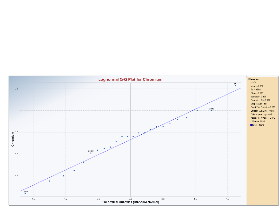
124
o The default GOF Method is Shapiro-Wilk.
o The default option for Graphs by Group is Group Graphs. If you want to see the
plots for all selected variables individually, and then check the button next to
Individual Graphs.
o Click OK button to continue or Cancel button to cancel the GOF tests.
Notes: This option for Graphs by Group is specifically provided for when the user wants to display
multiple graphs for a variable by a group variable (e.g., site AOC1, site AOC2, background). This kind of
display represents a useful visual comparison of the values of a variable (e.g., concentrations of COPC-
Arsenic) collected from two or more groups (e.g., upgradient wells, monitoring wells, residential wells).
Example 8-1a Consider the chromium concentrations data set used in Example 1-1 of Chapter 1. The
lognormal and normal GOF test results on chromium concentrations are shown in the following figures.
Output Screen for Lognormal Distribution (Full (w/o NDs))
Selected Options: Shapiro-Wilk
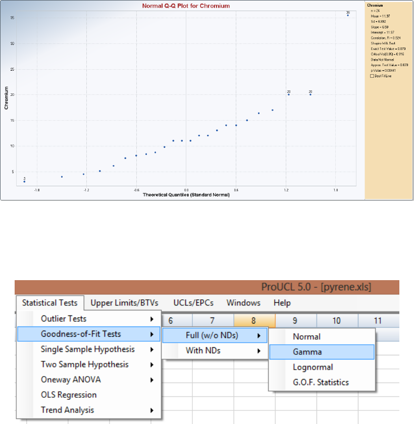
125
Output Screen for Normal Distribution (Full (w/o NDs))
Selected Options: Shapiro-Wilk, Best Fit Line not Displayed
8.2.2 GOF Tests for Gamma Distribution
1. Click Goodness-of-Fit Tests ► Full (w/o NDs) ► Gamma
2. The Select Variables screen (described in Chapter 3) will appear.
Select one or more variable(s) from the Select Variables screen.
If graphs have to be produced by using a group variable, then select a group variable by
clicking the arrow below the Select Group Column (Optional) button. This will result
in a drop-down list of available variables. The user should select and click on an
appropriate variable representing a group variable.
When the option button is clicked, the following window will be shown.
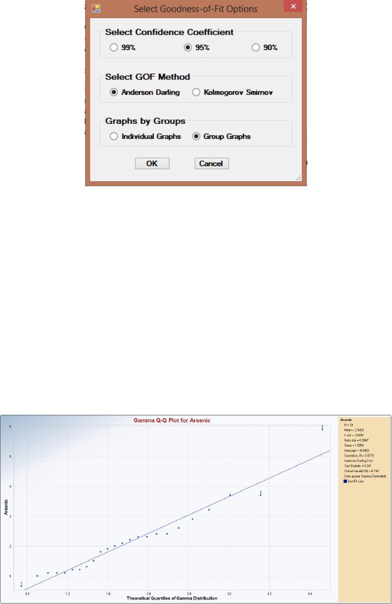
126
o The default option for the Confidence Coefficient is 95%.
o The default GOF method is Anderson Darling.
o The default option for Graph by Groups is Group Graphs. If you want to see
individual graphs, then check the radio button next to Individual Graphs.
o Click the OK button to continue or the Cancel button to cancel the option.
o Click OK button to continue or Cancel button to cancel the GOF tests.
Example 8-1b. Consider arsenic concentrations data set used in Example 1-1 of Chapter 1. The
Gamma GOF test results for arsenic concentrations, are shown in the following G.O.F. Q-Q plot.
Output Screen for Gamma Distribution (Full (w/o NDs))
Selected Options: Anderson Darling with Best Line Fit
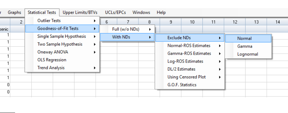
127
8.3 Goodness-of-Fit Tests Excluding NDs
This option is the most important option for a GOF test applied to data sets with ND observations. Based
upon the skewness and distribution of detected data, ProUCL computes the appropriate decision statistics
(UCLs, UPLs, UTLs, and USLs) which accommodate data skewness. Specifically, depending upon the
distribution of detected data, ProUCL uses KM estimates in parametric or nonparametric upper limits
computation formulae (UCLs, UTLs) to estimate EPC and BTV estimates.
1. Click Goodness-of-Fit Tests ► With NDs ► Exclude NDs
2. Select distribution to be tested: Normal, Gamma, or Lognormal.
To test for normality, click on Normal from the drop-down menu list.
To test for lognormality, click on Lognormal from the drop-down menu list.
To test for gamma distribution, click on Gamma from the drop-down menu list.
8.3.1 Normal and Lognormal Options
1. Click Goodness-of-Fit Tests ► With NDs ►Excluded NDs ► Normal or Lognormal
Note: In ProUCL 5.1, the censored probability plot option has been added as shown in the above drop-
down menu as "Using Censored Plot." This option is very much the same as the Q-Q plot option
generated by excluding NDs except that the hypothesized quantiles displayed along the x-axis adjust for
quantiles associated with NDs. There is not much difference (except for the correlation, slope and
intercept of the optional line displayed on the Q-Q plot) between these two graphs from the decision
making point of view. Censored probability (Q-Q) plots do not provide additional information than tools
and graphs already available in ProUCL 5.0. This was the reason that censored Q-Q plots were not
included in ProUCL 5.0 and its earlier versions.
2. The Select Variables screen (Chapter 3) will appear.
Select one or more variable(s) from the Select Variables screen.
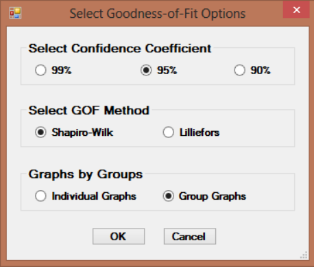
128
If graphs have to be produced by using a group variable, then select a group variable by
clicking the arrow below the Select Group Column (Optional) button. This will result
in a drop-down list of available variables. The user should select and click on an
appropriate variable representing a group variable.
When the option button: Normal or Lognormal is clicked, following window appears.
o The default option for the Confidence Coefficient is 95%.
o The default GOF Method is Shapiro-Wilk.
o The default option for Graphs by Group is Group Graphs. If you want to see the
plots for all selected variables individually, then check the button next to Individual
Graphs.
Click the OK button to continue or the Cancel button to cancel the option.
Click the OK button to continue or the Cancel button to cancel the GOF tests.
Example 8-2a. Consider the arsenic Oahu data set with NDs discussed in the literature (e.g.,
Helsel 2012; NADA in R [Helsel 2013]). The normal and lognormal GOF test results based upon
the detected data are shown in the following two figures. Censored Q-Q plots are also displayed
along with Q-Q plots based upon detected data.
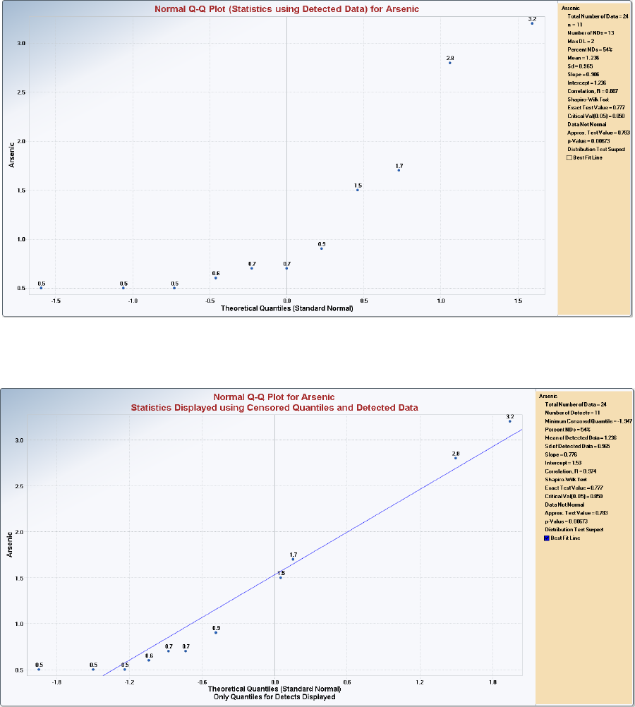
129
GOF Q-Q Plot for Normal Distribution (Exclude NDs)
Selected Options: Shapiro-Wilk
Censored Probability (Q-Q) Plot for Normal Distribution
Selected Options: Shapiro-Wilk and Best Line Fit
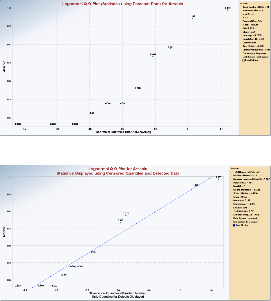
130
GOF Q-Q Plot for Lognormal Distribution (Exclude NDs)
Selected Options: Lilliefors Test
Censored Probability (Q-Q) Plot for Lognormal Distribution
Selected options: Lilliefors Test with Best Fit Line
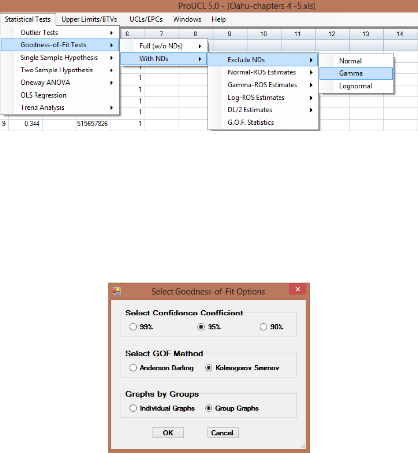
131
8.3.2 Gamma Distribution Option
1. Click Goodness-of-Fit Tests ► With NDs ►Excluded NDs ► Gamma
2. The Select Variables screen (Chapter 3) will appear.
Select one or more variable(s) from the Select Variables screen.
If graphs have to be produced by using a Group variable, then select a group variable by
clicking the arrow below the Select Group Column (Optional) button. This will result
in a drop-down list of available variables. The user should select and click on an
appropriate variable representing a group variable.
When the option button (Gamma) is clicked, the following window is shown.
o The default option for the Confidence Coefficient is 95%.
o The default GOF test method is the Anderson Darling test.
o The default option for Graph by Groups is Groups Graphs. If you want to
display all selected variables on separate graphs, check the button next to
Individual Graphs.
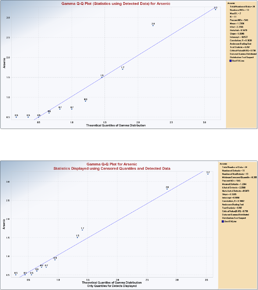
132
Click the OK button to continue or the Cancel button to cancel the option.
Click the OK button to continue or the Cancel button to cancel the GOF tests.
Example 8-2b (continued). Consider the arsenic Oahu data set with NDs as discussed in
Example 8-2a above. The gamma GOF test results based upon the detected data are shown in the
following GOF Q-Q plot.
Output Screen for Gamma Distribution (Exclude NDs)
Selected Options: Anderson-Darling Test with Best Fit Line
Censored Probability (Q-Q) Plot for Gamma Distribution
Selected options: Anderson-Darling Test with Best Fit Line
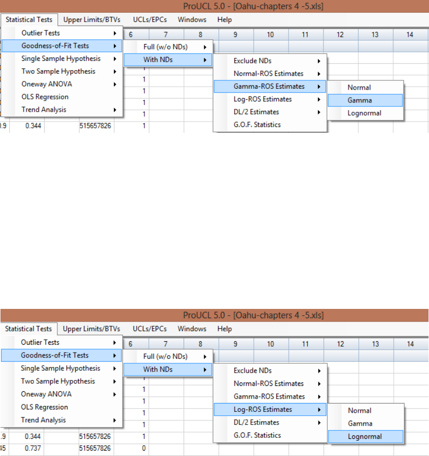
133
8.4 Goodness-of-Fit Tests with ROS Methods
1. Click Goodness-of-Fit Tests ► With NDs ► Gamma-ROS Estimates or Log-ROS Estimates
2. Select the distribution to be tested: Normal, Lognormal, or Gamma
To test for normal distribution, click on Normal from the drop-down menu list.
To test for gamma distribution, click on Gamma from the drop-down menu list.
To test for lognormal distribution, click on Lognormal from the drop-down menu.
8.4.1 Normal or Lognormal Distribution (Log-ROS Estimates)
1. Click Goodness-of-Fit Tests ► With NDs ► Log-ROS Estimates ► Normal, Lognormal
2. The Select Variables screen (Chapter 3) will appear.
Select one or more variable(s) from the Select Variables screen.
If graphs have to be produced by using a group variable, then select a group variable by
clicking the arrow below the Select Group Column (Optional) button. This will result
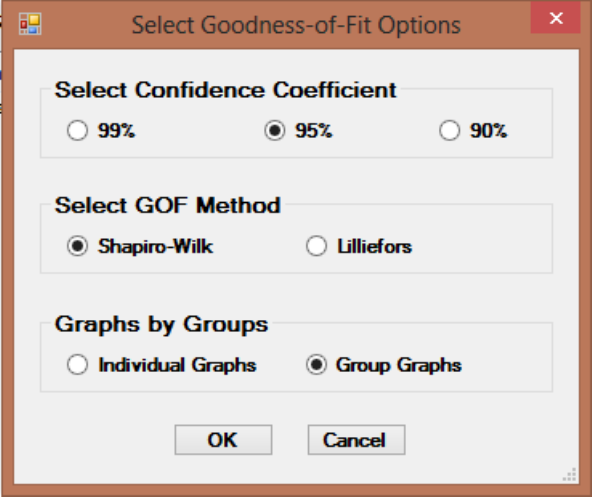
134
in a drop-down list of available variables. The user should select and click on an
appropriate variable representing a group variable.
When the option button: Normal or Lognormal is clicked, the following window appears.
o The default option for the Confidence Coefficient is 95%.
o The default GOF test Method is Shapiro-Wilk.
o The default option for Graphs by Group is Group Graphs. If you want to display
graphs for all selected variables individually, check the button next to Individual
Graphs.
Click the OK button to continue or the Cancel button to cancel the option.
Click the OK button to continue or the Cancel button to cancel the GOF tests.
Example 8-2c (continued). Consider the arsenic Oahu data set with NDs considered earlier in
this chapter. The lognormal GOF test results on LROS data (detected and imputed LROS NDs) is
shown in the following GOF Q-Q plot.
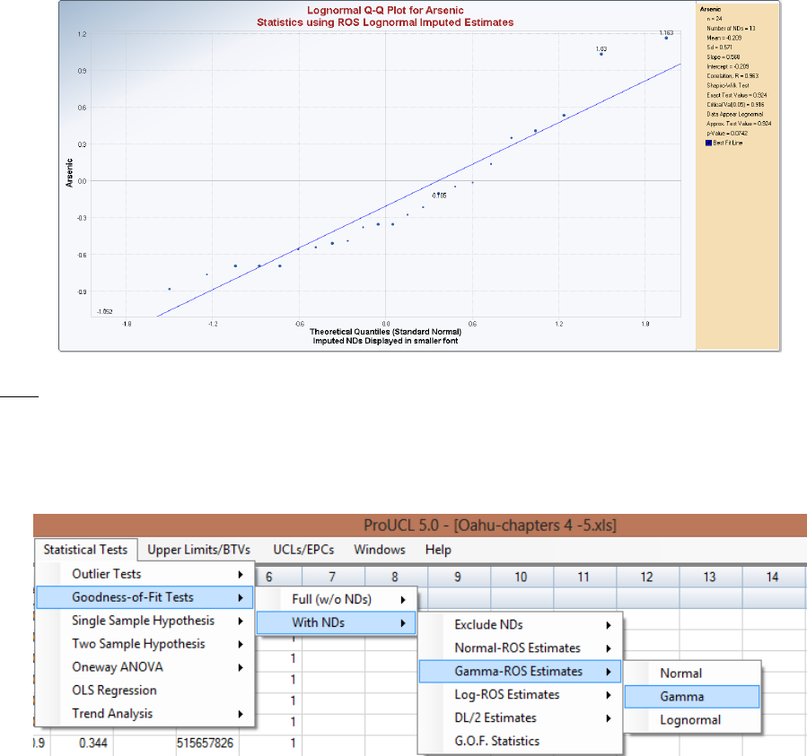
135
Output Screen for Lognormal Distribution (Log-ROS Estimates)
Selected Options: Shapiro Wilk test with Best Line Fit
Note: The font size of ND values is smaller than that of the detected values.
8.4.2 Gamma Distribution (Gamma-ROS Estimates)
1. Click Goodness-of-Fit Tests ► With NDs ► Gamma-ROS Estimates ► Gamma
2. The Select Variables screen (Chapter 3) will appear.
Select one or more variable(s) from the Select Variables screen.
If graphs have to be generated by using a Group variable, then select a group variable by
clicking the arrow below the Select Group Column (Optional) button. This will result
in a drop-down list of available variables. The user should select and click on an
appropriate variable representing a group variable.
When the option button (Gamma) is clicked, the following window will be shown.
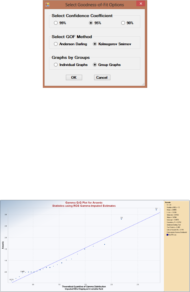
136
o The default option for the Confidence Coefficient is 95%.
o The default GOF test Method is Anderson Darling.
o The default option for Graph by Groups is Group Graphs. If you want to generate
separate graphs for all selected variables, the check the button next to Individual
Graphs.
Click the OK button to continue or the Cancel button to cancel the GOF tests.
Example 8-2d (continued). Consider the arsenic Oahu data set with NDs considered earlier. The
gamma GOF test results on GROS data (detected and imputed GROS NDs) are shown in the
following GOF Q-Q plot.
Output Screen for Gamma Distribution (Gamma-ROS Estimates)
Selected Options: Anderson Darling
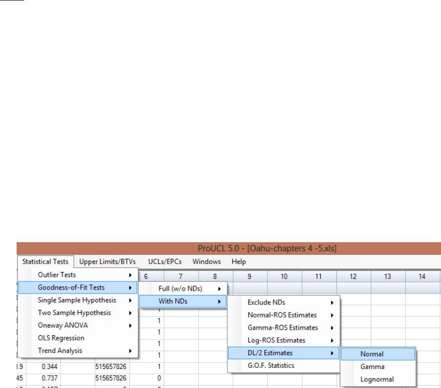
137
Note: The font size of ND values in the above graph (and in all GOF graphs) is smaller than that of
detected values.
8.5 Goodness-of-Fit Tests with DL/2 Estimates
1. Click Goodness-of-Fit Tests ► With NDs ► DL/2 Estimates
2. Select the distribution to be tested: Normal, Gamma, or Lognormal
To test for normality, click on Normal from the drop-down menu list.
To test for lognormality, click on Lognormal from the drop-down menu list.
To test for a gamma distribution, click on Gamma from the drop-down menu list.
8.5.1 Normal or Lognormal Distribution (DL/2 Estimates)
1. Click Goodness-of-Fit Tests ► With NDs ► DL/2 Estimates ► Normal or Lognormal
2. The Select Variables screen (Chapter 3) will appear.
Select one or more variable(s) from the Select Variables screen.
If graphs have to be generated by using a group variable, then select a group variable by
clicking the arrow below the Select Group Column (Optional) button. This will result
in a drop-down list of available variables. The user should select and click on an
appropriate variable representing a group variable.
The rest of the process to determine the distribution (normal, lognormal, and gamma) of the data
set thus obtained is the same as described in earlier sections.
8.6 Goodness-of-Fit Test Statistics
The G.O.F. option displays all GOF test statistics available in ProUCL. This option is used when the user
does not know which GOF test to use to determine the data distribution. Based upon the information
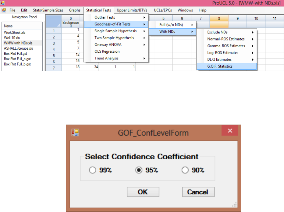
138
provided by the GOF test results, the user can perform an appropriate GOF test to generate GOF Q-Q plot
based upon the hypothesized distribution. This option is available for uncensored as well as left censored
data sets. Input and output screens associated with the G.O.F statistics option for data sets with NDs are
summarized as follows.
1. Click Goodness-of-Fit ► With NDs ► G.O.F. Statistics
2. The Select Variables screen (Chapter 3) will appear.
Select one or more variable(s) from the Select Variables screen.
When the option button is clicked, the following window will be shown.
The default confidence level is 95%.
Click the OK button to continue or the Cancel button to cancel the option.
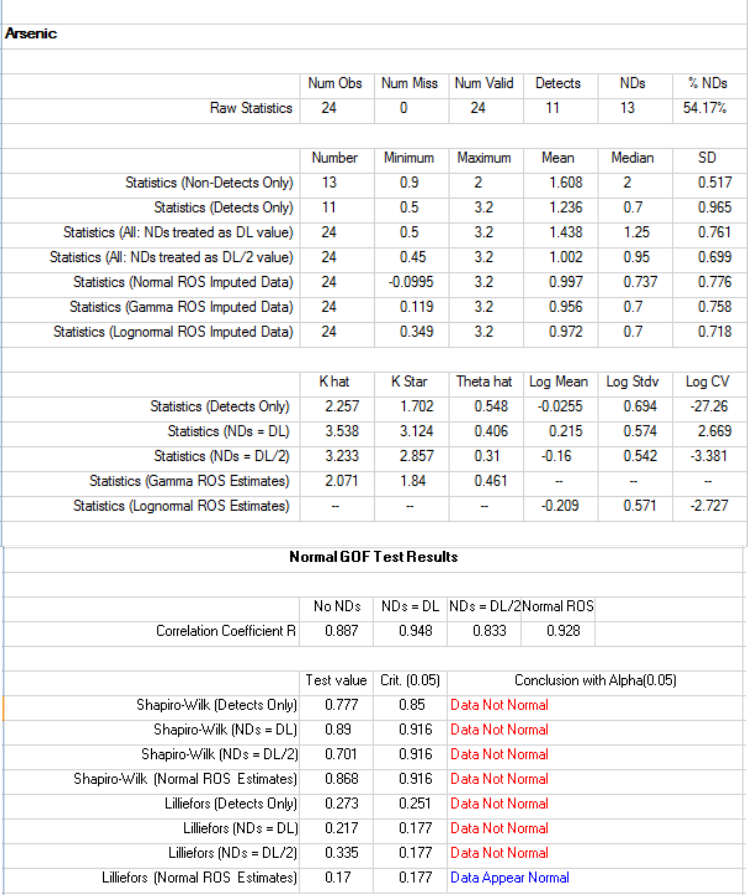
139
Example 8-2e (continued). Consider the arsenic Oahu data set with NDs discussed earlier. Partial GOF
test results, obtained using the G.O.F. Statistics option, are summarized in the following table.
Sample Output Screen for G.O.F. Test Statistics on Data Sets with Nondetect Observations
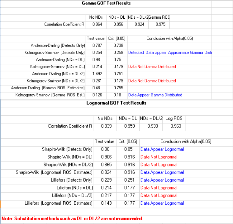
140
Sample Output Screen for G.O.F. Test Statistics on Data Sets with Nondetect Observations
(continued)
141
Chapter 9
Single-Sample and Two-Sample Hypotheses Testing Approaches
This chapter illustrates single-sample and two-sample parametric and nonparametric hypotheses testing
approaches as incorporated in the ProUCL software. All hypothesis tests are available under the
Statistical Tests module of ProUCL 5.0/ProUCL 5.1. ProUCL software can perform these hypotheses
tests on data sets with and without ND observations. It should be pointed out that, when one wants to use
two-sample hypotheses tests on data sets with NDs, ProUCL assumes that samples from both of the
samples/groups have ND observations. All this means is that, a ND column (with 0 or 1 entries only)
needs to be provided for the variable in each of the two samples. This has to be done even if one of the
samples (e.g., Site) has all detected entries; in this case the associated ND column will have all entries
equal to '1.' This will allow the user to compare two groups (e.g., arsenic in background vs. site samples)
with one of the groups having some NDs and the other group having all detected data.
9.1 Single-Sample Hypotheses Tests
In many environmental applications, single-sample hypotheses tests are used to compare site data with
pre-specified C
s
or CLs. The single-sample hypotheses tests are useful when the environmental
parameters such as the C
s
, action level, or CLs are known, and the objective is to compare site
concentrations with those known pre-established threshold values. Specifically, a t-test (or a sign test)
may be used to verify the attainment of cleanup levels at an AOC after a remediation activity; and a test
for proportion may be used to verify if the proportion of exceedances of an action level (or a compliance
limit) by sample concentrations collected from an AOC (or a MW) exceeds a certain specified proportion
(e.g., 1%, 5%, 10%).
ProUCL 5.1 can perform these hypotheses tests on data sets with and without ND observations.
However, it should be noted that for single-sample hypotheses tests (e.g., sign test, proportion test) used
to compare site mean/median concentration level with a C
s
or a CL (e.g., proportion test), all NDs (if any)
should lie below the cleanup standard, C
s.
For proper use of these hypotheses testing approaches, the
differences between these tests should be noted and understood. Specifically, a t-test or a Wilcoxon
Signed Rank (WSR) test is used to compare the measures of location and central tendencies (e.g., mean,
median) of a site area (e.g., AOC) to a cleanup standard, C
s
, or action level also representing a measure of
central tendency (e.g., mean, median); whereas, a proportion test compares if the proportion of site
observations from an AOC exceeding a CL exceeds a specified proportion, P
0
(e.g., 5%, 10%). ProUCL
has graphical methods that may be used to visually compare the concentrations of a site AOC with an
action level. This can be done using a box plot of site data with horizontal lines displayed at action levels
on the same graph. The details of the various single-sample hypotheses testing approaches are provided in
the associated ProUCL Technical Guide.

142
9.1.1 Single-Sample Hypothesis Testing for Full Data without Nondetects
1. Click Single Sample Hypothesis ► Full (w/o NDs)
2. Select Full (w/o NDs) – This option is used for full data sets without nondetects.
To perform a t-test, click on t-Test from the drop-down menu as shown above.
To perform a Proportion test, click on Proportion from the drop-down menu.
To run a Sign test, click on Sign test from the drop-down menu.
To run a Wilcoxon Signed Rank (WSR) test, click on Wilcoxon Signed Rank from the
drop-down menu.
All single-sample hypothesis tests for uncensored and left-censored data sets can be performed by
a group variable. The user selects a group variable by clicking the arrow below the Select Group
Column (Optional) button. This will result in a drop-down list of available variables. The user
should select and click on an appropriate variable representing a group variable.
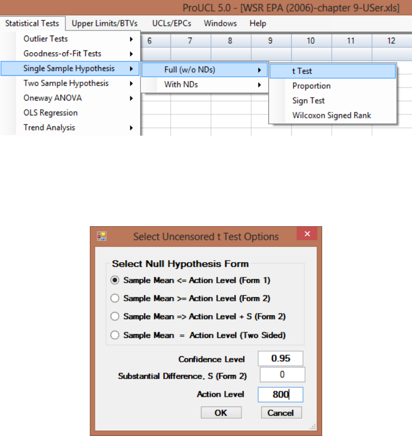
143
9.1.1.1 Single-Sample t-Test
1. Click Single Sample Hypothesis ► Full (w/o NDs) ► t-Test
2. The Select Variables screen will appear.
Select variable(s) from the Select Variables screen.
When the Options button is clicked, the following window will be shown.
o Specify the Confidence Level; default is 0.95.
o Specify meaningful values for Substantial Difference, S and the Action Level. The
default choice for S is “0.”
o Select form of Null Hypothesis; default is Sample Mean <= Action Level (Form 1).
o Click on OK button to continue or on Cancel button to cancel the test.
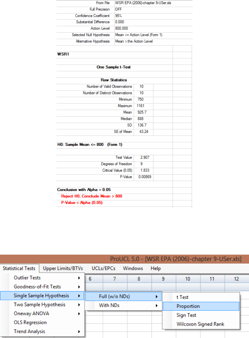
144
Example 9-1a. Consider the WSR data set described in EPA (2006a). One Sample t-test results
are summarized as follows.
Output for Single-Sample t-Test (Full Data w/o NDs)
9.1.1.2 Single-Sample Proportion Test
1. Click Single Sample Hypothesis ► Full (w/o NDs) ► Proportion
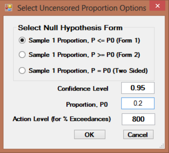
145
2. The Select Variables screen will appear.
Select variable(s) from the Select Variables screen.
When the Options button is clicked, the following window will be shown.
o Specify the Confidence level; default is 0.95.
o Specify the Proportion level and a meaningful Action Level.
o Select the form of Null Hypothesis; default is Sample 1 Proportion <= P0
(Form 1).
o Click on OK button to continue or on Cancel button to cancel the test.
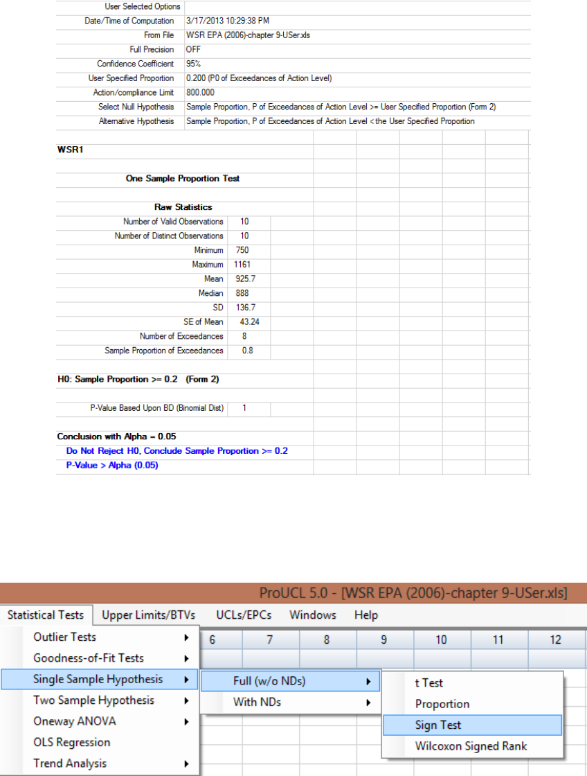
146
Example 9-1b (continued). Consider the WSR data set described in EPA (2006a). One Sample
proportion test results are summarized as follows.
Output for Single-Sample Proportion Test (Full Data without NDs)
9.1.1.3 Single-Sample Sign Test
1. Click Single Sample Hypothesis ► Full (w/o NDs) ► Sign test
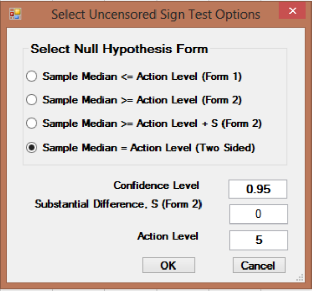
147
2. The Select Variables screen will appear.
Select variable(s) from the Select Variables screen.
When the Options button is clicked, the following window will be shown.
o Specify the Confidence Level; default choice is 0.95.
o Specify meaningful values for Substantial Difference, S and Action Level.
o Select the form of Null Hypothesis; default is Sample Median <= Action Level
(Form 1).
o Click on OK button to continue or on Cancel button to cancel the test.
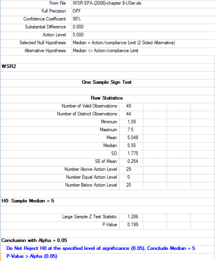
148
Example 9-1c (continued). Consider the WSR data set described in EPA (2006a). The Sign test
results are summarized as follows.
Output for Single-Sample Sign Test (Full Data without NDs)
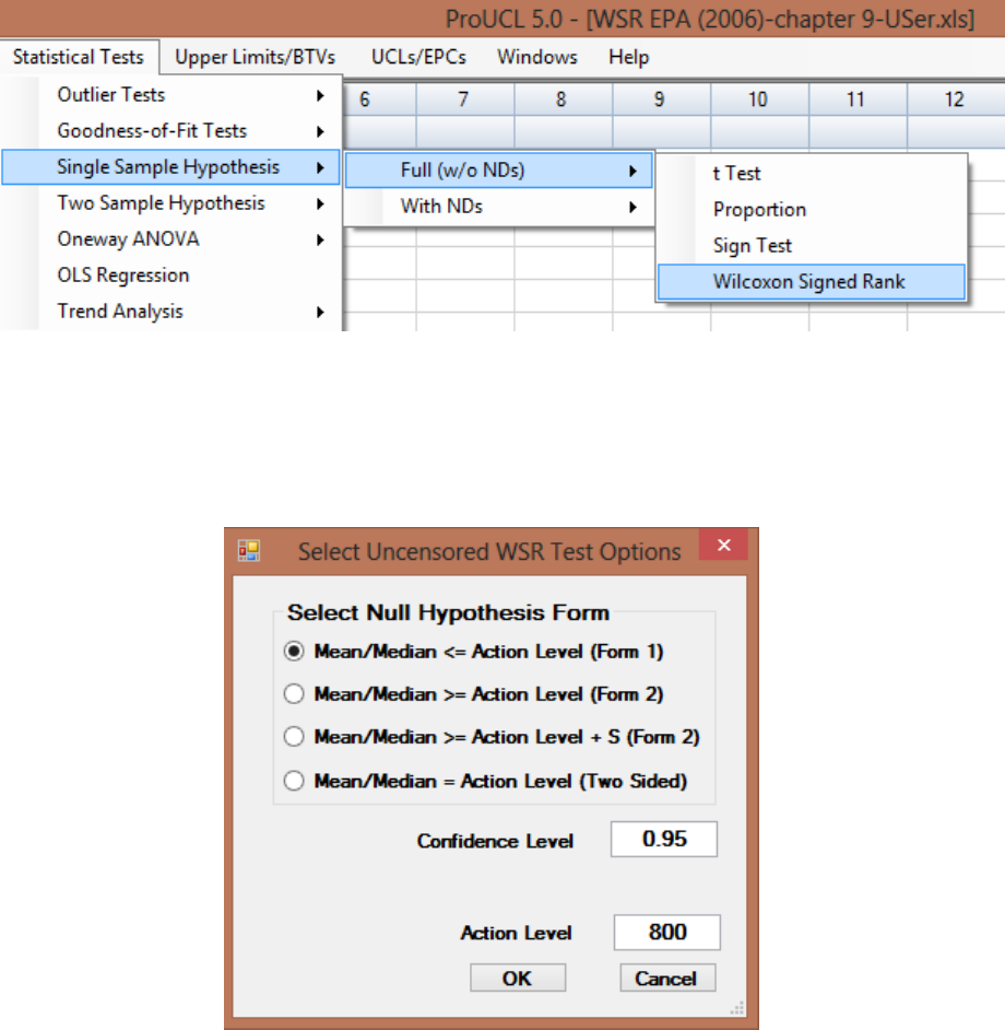
149
9.1.1.4 Single-Sample Wilcoxon Signed Rank (WSR) Test
1. Click Single Sample Hypothesis ► Full (w/o NDs) ► Wilcoxon Signed Rank
2. The Select Variables screen will appear.
Select variable(s) from the Select Variables screen.
When the Options button is clicked, the following window will be shown.
o Specify the Confidence Level; default is 0.95.
o Specify meaningful values for Substantial Difference, S, and Action Level.
o Select form of Null Hypothesis; default is Mean/Median <= Action Level (Form 1).
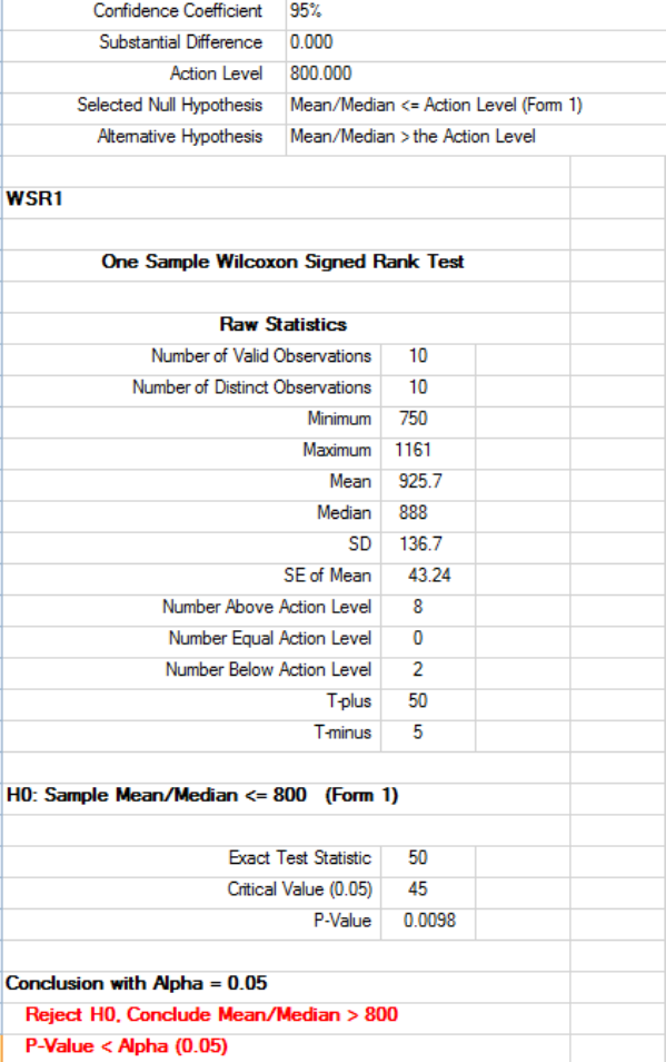
150
o Click on OK button to continue or on Cancel button to cancel the test.
Example 9-1d (continued). Consider the WSR data set described in EPA (2006a). One Sample
WSR test results are summarized as follows.
Output for Single-Sample Wilcoxon Signed Rank Test (Full Data without NDs)
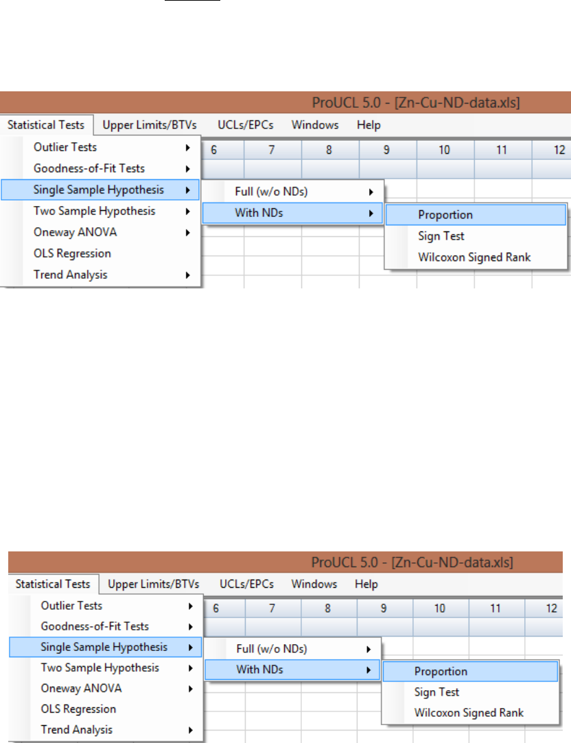
151
9.1.2 Single-Sample Hypothesis Testing for Data Sets with Nondetects
Most of the one-sample tests such as the Proportion test and the Sign test on data sets with ND values
assume that all ND observations lie below the specified action level, A
0
. These single-sample tests are not
performed if ND observations exceed the action levels. Single-sample hypothesis tests for data sets with
NDs are shown in the following screen shot.
1. Click on Single Sample Hypothesis ► With NDs
2. Select the With NDs option
To perform a proportion test, click on Proportion from the drop-down menu.
To perform a sign test, click on Sign test from the drop-down menu.
To perform a Wilcoxon Signed Rank test, click on Wilcoxon Signed Rank from the
drop-down menu list.
9.1.2.1 Single Proportion Test on Data Sets with NDs
1. Click Single Sample Hypothesis ► With NDs ► Proportion
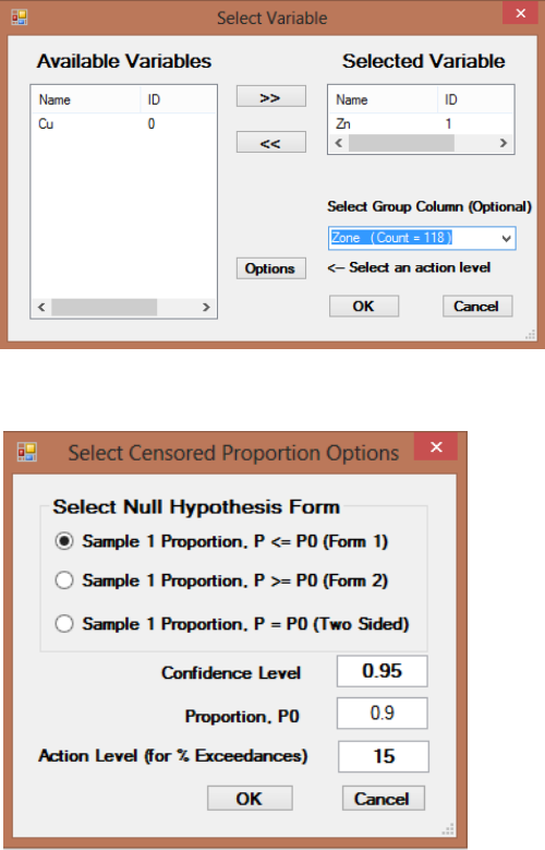
152
2. The Select Variables screen will appear.
Select variable(s) from the Select Variables screen.
If hypothesis test has to be performed by using a Group variable, then select a group
variable by clicking the arrow below the Select Group Column (Optional) button. This
will result in a drop-down list of available variables. The user should select and click on
an appropriate variable representing a group variable. This option has been used in the
following screen shot for the single-sample proportion test.
When the Options button is clicked, the following window will be shown.
o Specify the Confidence Level; default is 0.95.
o Specify meaningful values for Proportion and the Action Level (=15 here).
o Select form of Null Hypothesis; default is Sample 1 Proportion, P <= P0 (Form 1).
o Click on OK button to continue or on Cancel button to cancel the test.
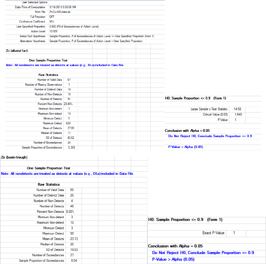
153
Example 9-2a. Consider the copper and zinc data set collected from two zones: Alluvial Fan and Basin
Trough discussed in the literature (Helsel 2012, NADA in R [Helsel 2013]). This data set is used here to
illustrate the one sample proportion test on a data set with NDs. The output sheet generated by ProUCL
5.1 is presented below.
Output for Single-Sample Proportion Test (with NDs) by Groups: Alluvial Fan and Basin Trough
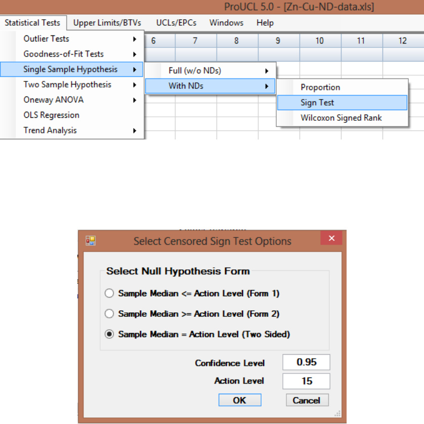
154
9.1.2.2 Single-Sample Sign Test with NDs
1. Click Single Sample Hypothesis ► With NDs ► Sign test
2. The Select Variables screen will appear.
Select variable(s) from the Select Variables screen.
When the Options button is clicked, the following window will be shown.
o Specify the Confidence Level; default is 0.95.
o Select an Action Level.
o Select the form of Null Hypothesis; default is Sample Median <= Action Level
(Form 1).
o Click on OK button to continue or on Cancel button to cancel the test.
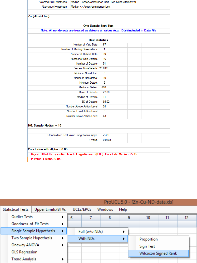
155
Example 9-2b (continued). Consider the copper and zinc data set collected from two zones: Alluvial Fan
and Basin Trough discussed above. This data set is used here to illustrate the Single-Sample Sign test on
a data set with NDs. The output sheet generated by ProUCL 5.0 follows.
Output for Single-Sample Sign Test (Data with Nondetects)
9.1.2.3 Single-Sample Wilcoxon Signed Rank Test with NDs
1. Click Single Sample Hypothesis ► With NDs ► Wilcoxon Signed Rank
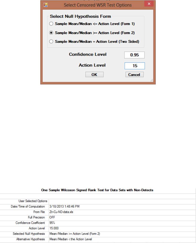
156
2. The Select Variables screen will appear.
Select variable(s) from the Select Variables screen.
When the Options button is clicked, the following window will be shown.
o Specify the Confidence Level; default is 0.95.
o Specify an Action Level.
o Select form of Null Hypothesis; default is Sample Mean/Median <= Action Level
(Form 1).
o Click on OK button to continue or on Cancel button to cancel the test.
Example 9-2c (continued). Consider the copper and zinc data set collected from two zones: Alluvial Fan
and Basin Trough discussed earlier in this chapter. This data set is used here to illustrate one sample
Wilcoxon Signed Rank test on a data set with NDs. The output sheet generated by ProUCL 5.0 is
provided as follows.
Output for Single-Sample Wilcoxon Signed Rank Test (Data with Nondetects)
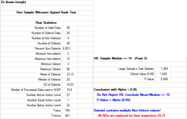
157
Output for Single-Sample Wilcoxon Signed Rank Test (Data with Nondetects)- continued
9.2 Two-Sample Hypotheses Testing Approaches
The two-sample hypotheses testing approaches available in ProUCL are described in this section. Like
Single-Sample Hypothesis, the Two-Sample Hypothesis options are available under the Statistical
Tests module of ProUCL 5.0/ProUCL 5.1. These approaches are used to compare the parameters and
distributions of two populations (e.g., Background vs. AOC) based upon data sets collected from those
populations. Several forms (Form 1 and Form 2, and Form 2 with Substantial Difference, S) of the two-
sample hypothesis testing approaches are available in ProUCL. The methods are available for full-
uncensored data sets as well as for data sets with ND observations with multiple detection limits.
Full (w/o NDs) – performs parametric and nonparametric hypothesis tests on uncensored data
sets consisting of all detected values. The following tests are available:
o Student’s t and Satterthwaite tests to compare the means of two populations (e.g.
Background versus AOC).
o F-test to the check the equality of dispersions of two populations.
o Two-sample nonparametric Wilcoxon-Mann-Whitney (WMW) test. This test is
equivalent to Wilcoxon Rank Sum (WRS) test.
With NDs – performs hypothesis tests on left-censored data sets consisting of detected and
ND values. The following tests are available:
o Wilcoxon-Mann-Whitney test. All observations (including detected values) below the
highest detection limit are treated as ND (less than the highest DL) values.

158
o Gehan’s test is useful when multiple detection limits may be present.
o Tarone-Ware test is useful when multiple detection limits may be present.
The details of these methods can be found in the ProUCL Technical Guides (2013, 2015) and are also
available in EPA (2002b, 2006a, 2009a, 2009b). It is emphasized that the use of informal graphical
displays (e.g., side-by-side box plots, multiple Q-Q plots) should always accompany the formal
hypothesis testing approaches listed above. This is especially warranted when data sets may consist of
NDs with multiple detection limits and observations from multiple populations (e.g., mixture samples
collected from various onsite locations) and outliers.
Notes: As mentioned before, when one wants to use two-sample hypotheses tests on data sets with NDs,
ProUCL assumes that samples from both of the groups have ND observations. This may not be the case,
as data from a polluted site may not have any ND observations. ProUCL can handle such data sets; the
user will have to provide a ND column (with 0 or 1 entries only) for the selected variable of each of the
two samples/groups. Thus when one of the samples (e.g., site arsenic) has no ND value, the user supplies
an associated ND column with all entries equal to '1'. This will allow the user to compare two groups
(e.g., arsenic in background vs. site samples) with one of the groups having some NDs and the other
group having all detected data.
9.2.1 Two-Sample Hypothesis Tests for Full Data
Full (w/o NDs): This option is used to analyze data sets consisting of all detected values. The following
two-sample tests are available in ProUCL 5.1.
Student’s t and Satterthwaite tests to compare the means of two populations (e.g.,
Background versus AOC).
F-test is also available to test the equality of dispersions of two populations.
Two-sample nonparametric Wilcoxon-Mann-Whitney (WMW) test.
Student’s t-Test
o Based upon collected data sets, this test is used to compare the mean concentrations of
two populations/groups provided the populations are normally distributed. The data sets
are represented by independent random observations, X1, X2, . . . , Xn collected from one
population (e.g., site), and independent random observations, Y1, Y2, . . . , Ym collected
from another (e.g., background) population. The same terminology is used for all other
two-sample tests discussed in the following sub-sections of this section.
o Student’s t-test also assumes that the spreads (variances) of the two populations are
approximately equal.
o The F-test can be used to the check the equality of dispersions of two populations. A
couple of other tests (e.g., Levene 1960) are also available in the literature to compare the
variances of two populations. Since the F-test performs fairly well, other tests are not
included in the ProUCL software. For more details refer to ProUCL Technical Guides.
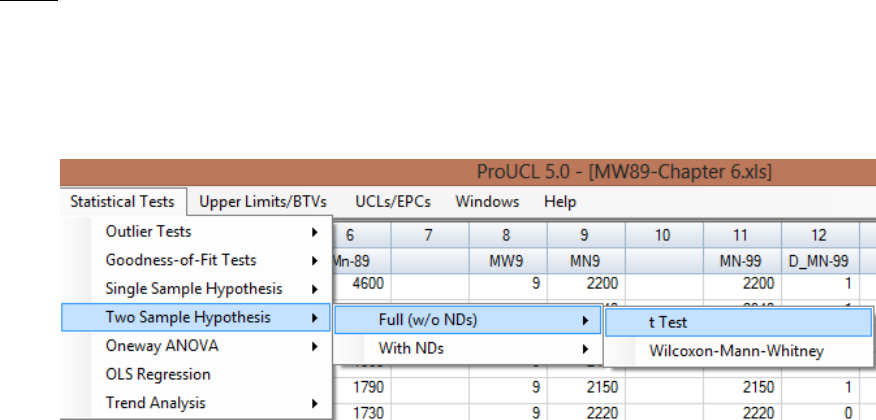
159
Satterthwaite t-Test
This test is used to compare the means of two populations when the variances of those
populations may not be equal. As mentioned before, the F-distribution based test can be
used to verify the equality of dispersions of the two populations. However, this test alone
is more powerful test to compare the means of two populations.
Test for Equality of two Dispersions (F-test)
o This test is used to determine whether the true underlying variances of two populations
are equal. Usually the F-test is employed as a preliminary test, before conducting the two-
sample t-test for testing the equality of means of two populations.
o The assumptions underlying the F-test are that the two-samples represent independent
random samples from two normal populations. The F-test for equality of variances is
sensitive to departures from normality.
Two-Sample Nonparametric WMW Test
o This test is used to determine the comparability of the two continuous data distributions.
This test also assumes that the shapes (e.g., as determined by spread, skewness, and
graphical displays) of the two populations are roughly equal. The test is often used to
determine if the measures of central locations (mean, median) of the two populations are
significantly different.
o The Wilcoxon-Mann-Whitney test does not assume that the data are normally or log-
normally distributed. For large samples (e.g., 20), the distribution of the WMW test
statistic can be approximated by a normal distribution.
Notes: The use of the tests listed above is not recommended on log-transformed data sets, especially when
the parameters of interests are the population means. In practice, cleanup and remediation decisions have
to be made in the original scale based upon statistics and estimates computed in the original scale. The
equality of means in log-scale does not necessarily imply the equality of means in the original scale.
1. Click on Two Sample Hypothesis ► Full (w/o NDs)
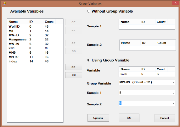
160
2. Select the Full (w/o NDs) option
To perform a t-test, click on t Test from the drop-down menu.
To perform a Wilcoxon-Mann-Whitney, click on Wilcoxon-Mann-Whitney from the
drop-down menu list.
9.2.1.1 Two-Sample t-Test without NDs
1. Click on Two Sample Hypothesis ► Full (w/o NDs) ► t Test
2. The Select Variables screen will appear.
Select variable(s) from the Select Variables screen.
Without Group Variable: This option is used when the sampled data of the variable
(e.g., lead) for the two populations (e.g., site vs. background) are given in separate
columns.
With Group Variable: This option is used when sampled data of the variable (e.g., lead)
for the two populations (e.g., site vs. background) are given in the same column.
The values are separated into different populations (groups) by the values of an
associated Group ID Variable. The group variable may represent several populations
(e.g., background, surface, subsurface, silt, clay, sand, several AOCs, MWs). The user
can compare two groups at a time by using this option.
When the Group option is used, the user then selects a variable by using the Group
Variable Option. The user should select an appropriate variable representing a group
variable. The user can use letters, numbers, or alphanumeric labels for the group names.
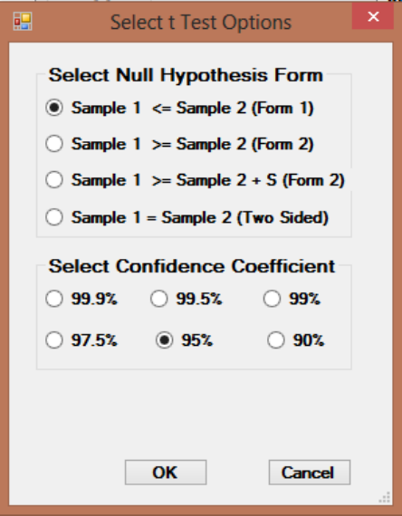
161
o When the Options button is clicked, the following window will be shown.
o Specify a useful Substantial Difference, S value. The default choice is 0.
o Select the Confidence Coefficient. The default choice is 95%.
o Select the form of Null Hypothesis. The default is Sample 1 <= Sample 2 (Form 1).
o Click on OK button to continue or on Cancel button to cancel the option.
Click on OK button to continue or on Cancel button to cancel the Sample 1 versus
Sample 2 Comparison.
Example 9-3. Consider the manganese concentrations data set collected from three wells: MW1, an
upgradient well, and MW8 and MW9, two downgradient wells. The two-sample t-test results, comparing
Mn concentrations in MW8 vs. MW9, are described as follows.
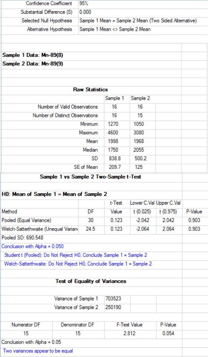
162
Output for Two-Sample t-Test (Full Data without NDs)
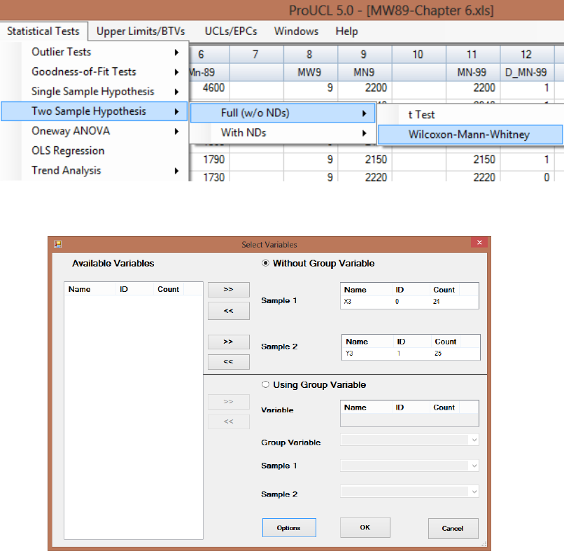
163
9.2.1.2 Two-Sample Wilcoxon-Mann-Whitney (WMW) Test without NDs
1. Click on Two Sample Hypothesis Testing ► Full (w/o NDs) ► Wilcoxon-Mann-Whitney
2. The Select Variables screen will appear.
Select variable(s) from the Select Variables screen.
Without Group Variable: This option is used when the data values of the variable
(arsenic) are given in separate columns.
With Group Variable: This option is used when data of the variable (arsenic) are given
in the same column. The values are separated into different samples (groups) by the
values of an associated Group Variable.
When the Group option is used, the user then selects a group variable/ID by using the
Group Variable Option. The user should select an appropriate variable representing a
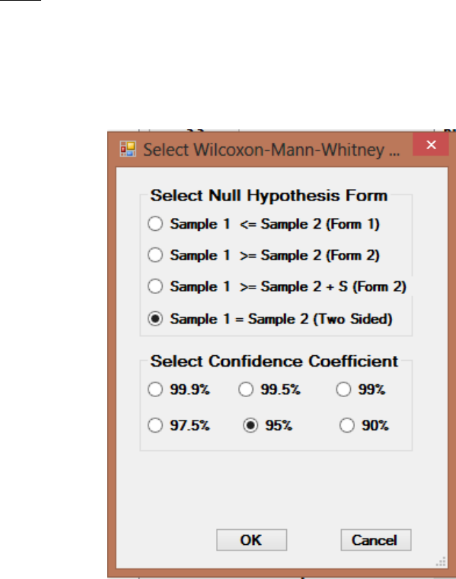
164
group variable. The user can use letters, numbers, or alphanumeric labels for the group
names.
Notes: ProUCL documents have been written using environmental terminology such as
performing background versus site comparisons. However, all tests and procedures incorporated
in ProUCL can be used on data sets from any other application. For other applications such as
comparing a new treatment drug versus older treatment drug, the group variable may represent
the two groups: Control Drug and New Drug.
When the Options button is clicked, the following window is shown.
o Specify a Substantial Difference, S value. The default choice is 0.
o Choose the Confidence Coefficient. The default choice is 95%.
o Select the form of Null Hypothesis. The default is Sample 1<= Sample 2 (Form 1).
o Click on OK button to continue or on Cancel button to cancel the selected options.
Click on OK to continue or on Cancel to cancel Sample 1 vs. Sample 2 comparison.
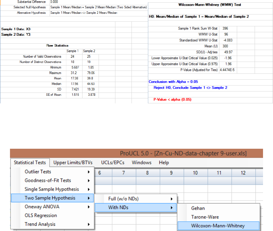
165
Example 9- 4. The two-sample Wilcoxon Mann Whitney (WMW) test results on a data set with ties are
summarized as follows.
Output for Two-Sample Wilcoxon-Mann-Whitney Test (Full Data with ties)
9.2.2 Two-Sample Hypothesis Testing for Data Sets with Nondetects
1. Click Two Sample Hypothesis ► With NDs
2. Select the With NDs option. A list of available tests will appear (shown above).
To perform a Wilcoxon-Mann-Whitney test, click on Wilcoxon-Mann-Whitney from
the drop-down menu list.
To perform a Gehan test, click on Gehan from the drop-down menu.
To perform a Tarone-Ware test, click on Tarone-Ware from the drop-down menu.
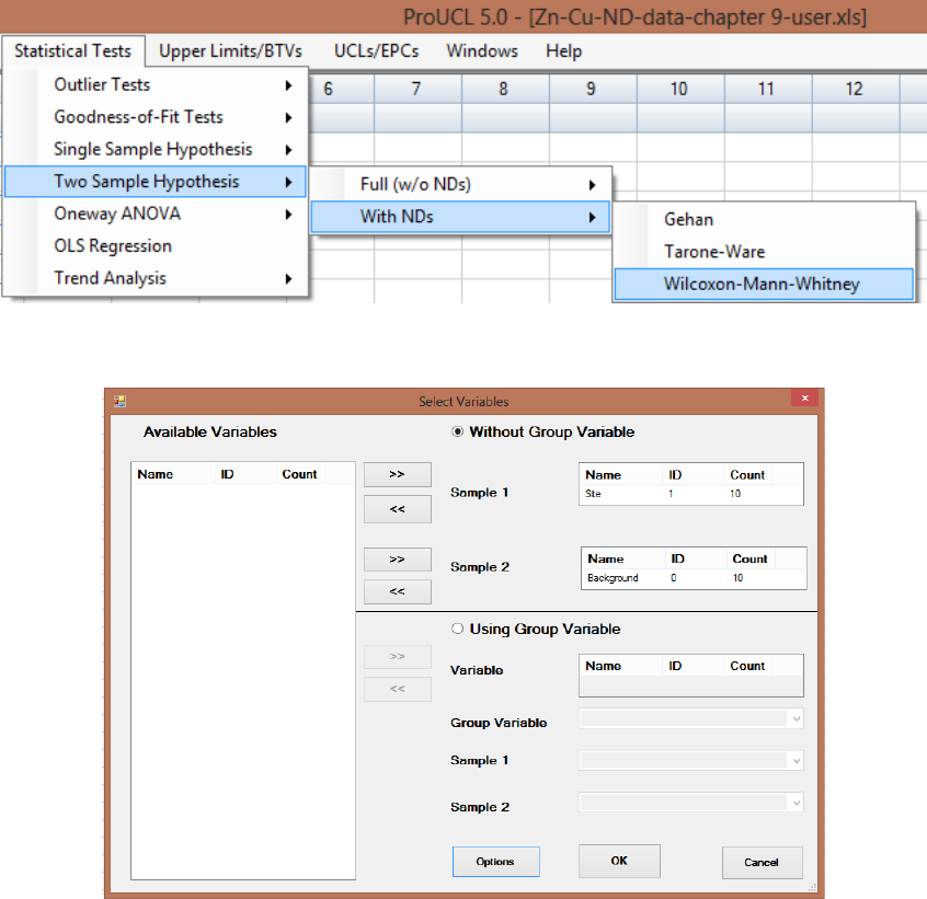
166
9.2.2.1 Two-Sample Wilcoxon-Mann-Whitney Test with Nondetects
1. Click Two Sample Hypothesis ► With NDs ► Wilcoxon-Mann-Whitney
2. The Select Variables screen shown below will appear.
Select variable(s) from the Select Variables screen.
Without Group Variable: This option is used when the data values of the variable (e.g.,
TCDD 2,3,7,8) for the site and the background are given in separate columns.
With Group Variable: This option is used when data values of the variable (TCDD 2, 3,
7, 8) are given in the same column. The values are separated into different samples
(groups) by the values of an associated Group Variable. When using this option, the
user should select an appropriate variable representing groups such as AOC1, AOC2,
AOC3 etc.
When the Options button is clicked, the following window will be shown.
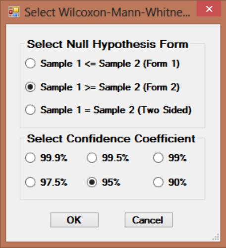
167
o Choose the Confidence Coefficient. The default choice is 95%.
o Select the form of Null Hypothesis. The default is Sample 1 <= Sample 2 (Form 1).
o Click on OK button to continue or on Cancel button to cancel the selected options.
Click on OK to continue or on Cancel to cancel the Sample 1 vs. Sample 2 comparison.
Example 9-5. Consider a two sample data set with nondetects and multiple detection limits. Since the
data sets have more than one detection limit, the WMW test is not recommended for this data set.
However, sometimes, the users tend to use the WMW test on data sets with multiple detection limits. The
WMW test results are summarized as follows.
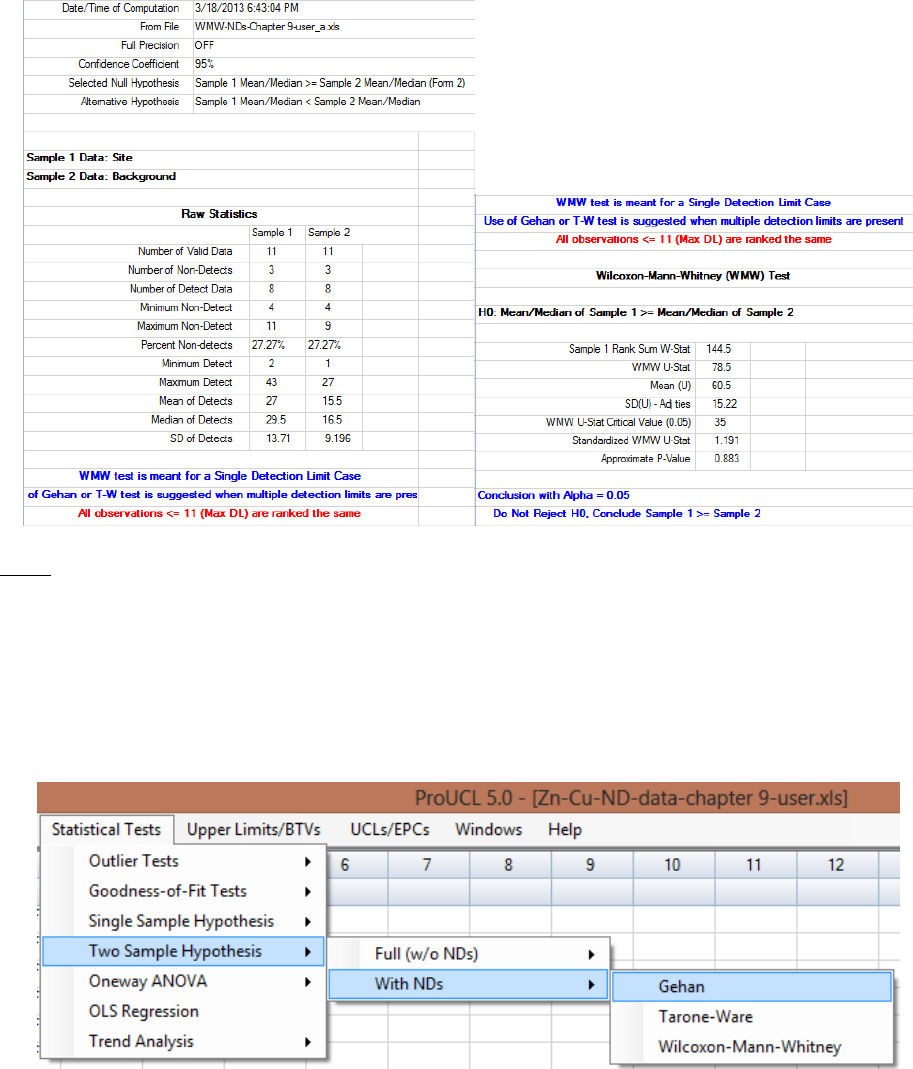
168
Output for Two-Sample Wilcoxon-Mann-Whitney Test (with Nondetects)
Notes: In the WMW test, all observations below the largest detection limit are considered as NDs
(potentially including some detected values) and hence they all receive the same average rank. This action
tends to reduce the associated power of the WMW test considerably. This in turn may lead to an incorrect
conclusion.
9.2.2.2 Two-Sample Gehan Test for Data Sets with Nondetects
1. Click Two Sample Hypothesis ► With NDs ► Gehan
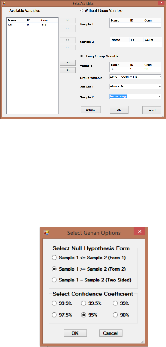
169
2. The Select Variables screen will appear.
Select variable(s) from the Select Variables screen.
Without Group Variable: This option is used when the data values of the variable
(Zinc) for the two data sets are given in separate columns.
With Group Variable: This option is used when data values of the variable (Zinc) for
the two data sets are given in the same column. The values are separated into different
samples (groups) by the values of an associated Group Variable. When using this
option, the user should select a group variable representing groups/populations such as
Zone 1, Zone2, Zone3, etc.
When the Options button is clicked, the following window will be shown.
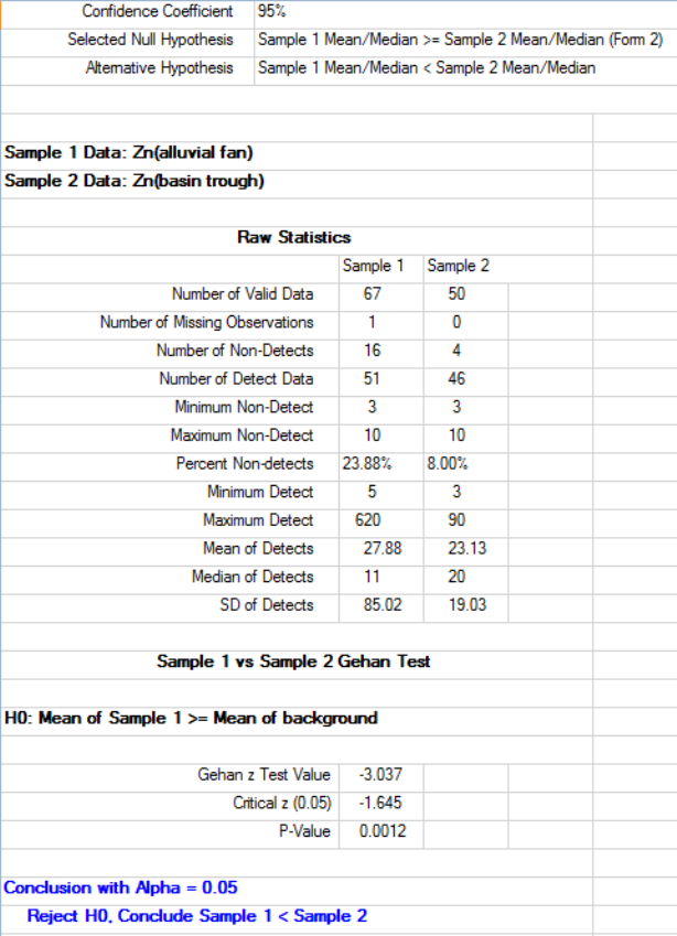
170
o Choose the Confidence Coefficient. The default choice is 95%.
o Select the form of Null Hypothesis. The default is Sample 1 <= Sample 2 (Form 1).
o Click on OK button to continue or on Cancel button to cancel selected options.
Click on the OK button to continue or on the Cancel button to cancel the Sample 1 vs.
Sample 2 Comparison.
Example 9-6a. Consider the copper and zinc data set collected from two zones: Alluvial Fan and Basin
Trough discussed in the literature (Helsel 2012). This data set is used here to illustrate the Gehan two-
sample test. The output sheet generated by ProUCL 5.0 (similar sheet is generated using ProUCL 5.1,
therefore the following output is not replaced) follows.
Output for Two-Sample Gehan Test (with Nondetects)
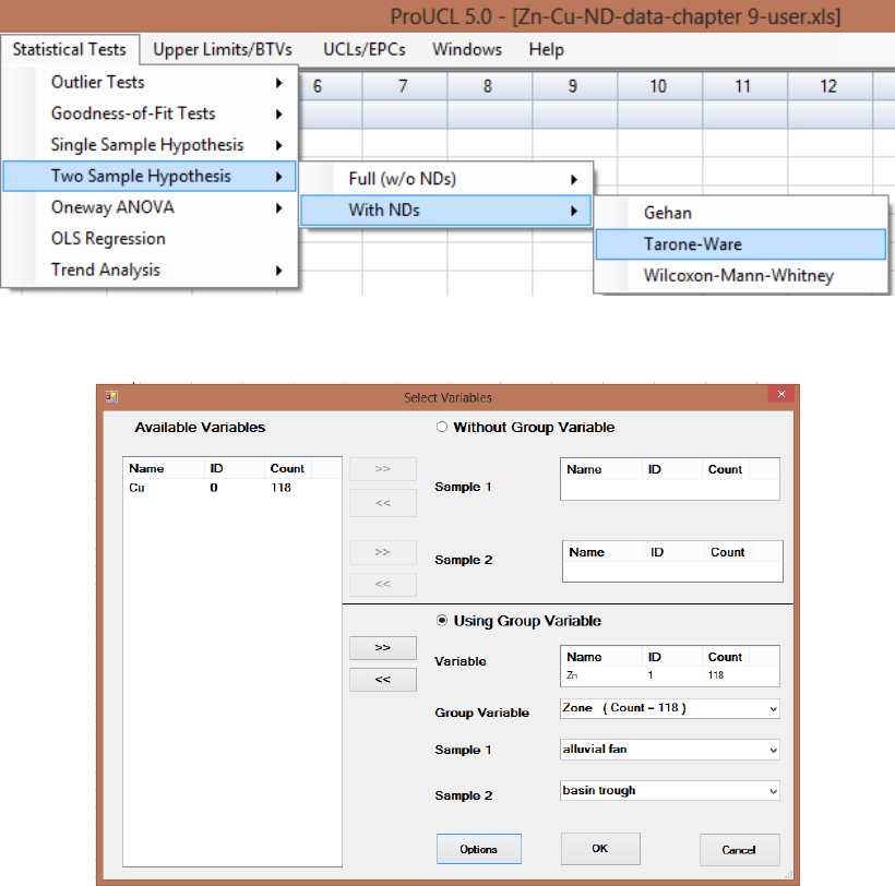
171
9.2.2.3 Two-Sample Tarone-Ware Test for Data Sets with Nondetects
The two-sample Tarone-Ware (T-W) test (1978) for data sets with NDs is new in ProUCL 5.0.
1. Click Two Sample Hypothesis Testing ► Two Sample ► With NDs ► Tarone-Ware
2. The Select Variables screen will appear.
Select variable(s) from the Select Variables screen.
Without Group Variable: This option is used when the data values of the variable (Cu)
for the two data sets are given in separate columns.
With Group Variable: This option is used when data values of the variable (Cu) for the
two data sets are given in the same column. The values are separated into different
samples (groups) by the values of an associated Group Variable. When using this
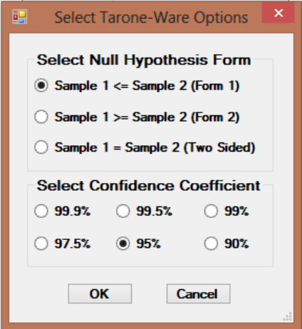
172
option, the user should select a group variable/ID by clicking the arrow next to the
Group Variable option for a drop-down list of available variables. The user selects an
appropriate group variable representing the groups to be tested.
When the Options button is clicked, the following window will be shown.
o Choose the Confidence Coefficient. The default choice is 95%.
o Select the form of Null Hypothesis. The default is Sample 1 <= Sample 2 (Form 1).
o Click on OK button to continue or on Cancel button to cancel selected options.
Click on the OK button to continue or on the Cancel button to cancel the Sample 1 vs.
Sample 2 Comparison.
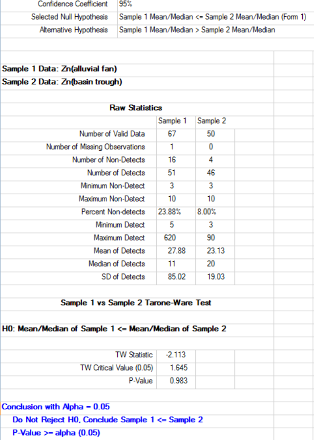
173
Example 9-6b (continued). Consider the copper and zinc data set used earlier. The data set is used here
to illustrate the T-W two-sample test. The output sheet generated by ProUCL 5.0/ProUCL 5.1 is
described as follows.
Output for Two-Sample Tarone-Ware Test (with Nondetects)
174

175
Chapter 10
Computing Upper Limits to Estimate Background Threshold
Values Based Upon Full Uncensored Data Sets and Left-
Censored Data Sets with Nondetects
This chapter illustrates the computations of parametric and nonparametric statistics and upper limits that
can be used as estimates of BTVs and other not-to-exceed values. The BTV estimation methods are
available for data sets with and without ND observations. Technical details about the computation of the
various limits can be found in the associated ProUCL 5.1 Technical Guide. For each selected variable,
this option computes various upper limits such as UPLs, UTLs, USLs and upper percentiles to estimate
the BTVs that are used in site versus background evaluations.
Two choices are available to compute background statistics for data sets:
Full (w/o NDs) – computes background statistics for uncensored full data sets without
any ND observation.
With NDs – computes background statistics for data sets consisting of detected as well as
nondetected observations with multiple detection limits.
The user specifies the confidence coefficient (probability) associated with each interval estimate. ProUCL
accepts a CC value in the interval [0.5, 1), 0.5 inclusive. The default choice is 0.95. For data sets with and
without NDs, ProUCL 5.0/ProUCL 5.1 can compute the following upper limits to estimate BTVs:
Parametric and nonparametric upper percentiles.
Parametric and nonparametric UPLs for a single observation, future or next k ( 1)
observations, mean of next k observations. Here future k, or next k observations may
represent k observations from another population (e.g., site) different from the sampled
(background) population.
Parametric and nonparametric UTLs.
Parametric and nonparametric USLs.
Note on Computing Lower Limits: In many environmental applications (e.g., groundwater monitoring),
one needs to compute lower limits including: lower prediction limits (LPLs), lower tolerance limits
(LTLs), or lower simultaneous limit (LSLs). At present, ProUCL does not directly compute a LPL, LTL,
or a LSL. It should be noted that for data sets with and without nondetects, ProUCL outputs several
intermediate results and critical values (e.g., khat, nuhat, K, d2max) needed to compute the interval
estimates and lower limits. For data sets with and without NDs, except for the bootstrap methods, the
same critical value (e.g., normal z value, Chebyshev critical value, or t-critical value) can be used to
compute a parametric LPL, LSL, or a LTL (for samples of size >30 to be able to use Natrella's
approximation in LTL) as used in the computation of a UPL, USL, or a UTL (for samples of size >30).
Specifically, to compute a LPL, LSL, and LTL (n>30) the '+' sign used in the computation of the
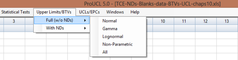
176
corresponding UPL, USL, and UTL (n>30) needs to be replaced by the '-' sign in the equations used to
compute UPL, USL, and UTL (n>30). For specific details, the user may want to consult a statistician. For
data sets without ND observations, the user may want to use the Scout 2008 software package (EPA
2009c) to compute the various parametric and nonparametric LPLs, LTLs (all sample sizes), and LSLs.
10.1 Background Statistics for Full Data Sets without Nondetects
1. Click Upper Limits/BTVs ► Full (w/o NDs)
2. Select Full (w/o NDs)
To compute background statistics assuming the normal distribution, click on Normal
from the drop-down menu list.
To compute background statistics assuming the gamma distribution, click on Gamma
from the drop-down menu list.
To compute background statistics assuming the lognormal distribution, click on
Lognormal from the drop-down menu list.
To compute background statistics using distribution-free nonparametric methods, click on
Non-Parametric from the drop-down menu list.
To compute and see all background statistics available in ProUCL, click on the All option
from the drop-down menu list. ProUCL will display data distribution, all parametric and
nonparametric background statistics in an Excel type spreadsheet. The user may use this
output sheet to select the most appropriate statistic to estimate a BTV.
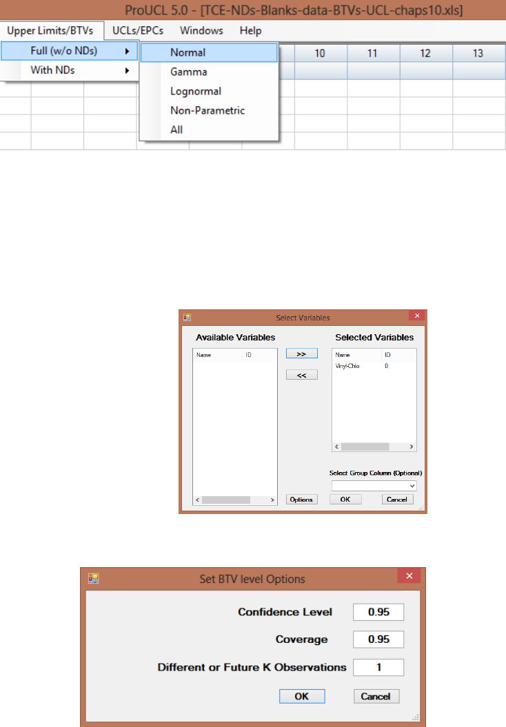
177
10.1.1 Normal or Lognormal Distribution
1. Click Upper Limits/BTVs ► Full (w/o NDs) ► Normal or Lognormal
2. The Select Variables screen (Chapter 3) will appear.
Select a variable(s) from the Select Variables screen.
To compute BTV estimates by a group variable, select a group variable by clicking the
arrow below the Select Group Column (Optional) to obtain a drop-down list of
available variables and select an appropriate group variable.
When the Option button is clicked, the following window will be shown.
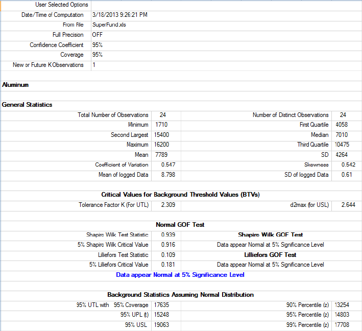
178
o Specify the Confidence Level; a number in the interval (0.5, 1), 0.5 inclusive. The
default choice is 0.95.
o Specify the Coverage coefficient (for a percentile) needed to compute UTLs.
Coverage represents a number in the interval (0.0, 1). The default choice is 0.95.
Remember, a UTL is an upper confidence limit (e.g., with confidence level = 0.95)
for a 95% (e.g., with coverage = 0.95) percentile.
o Specify the Different or Future K Observations. The default choice is 1. It is noted
that when K = 1, the resulting interval will be a UPL for a single future observation.
In the example shown above, a value of K = 1 has been used.
o Click on OK button to continue or on Cancel button to cancel this option.
Click on OK to continue or on Cancel button to cancel the Upper Limits/BTVs options.
Example 10-1a. Consider the real data set described in Example 1-1 of Chapter 1 collected from a
Superfund site. Aluminum concentrations follow a normal distribution and manganese concentrations
follow a lognormal distribution. The normal and lognormal distribution based estimates of BTVs are
summarized in the following two tables.
Aluminum - Output Screen for BTV Estimates Based upon a Normal Distribution
(Full - Uncensored Data Set)
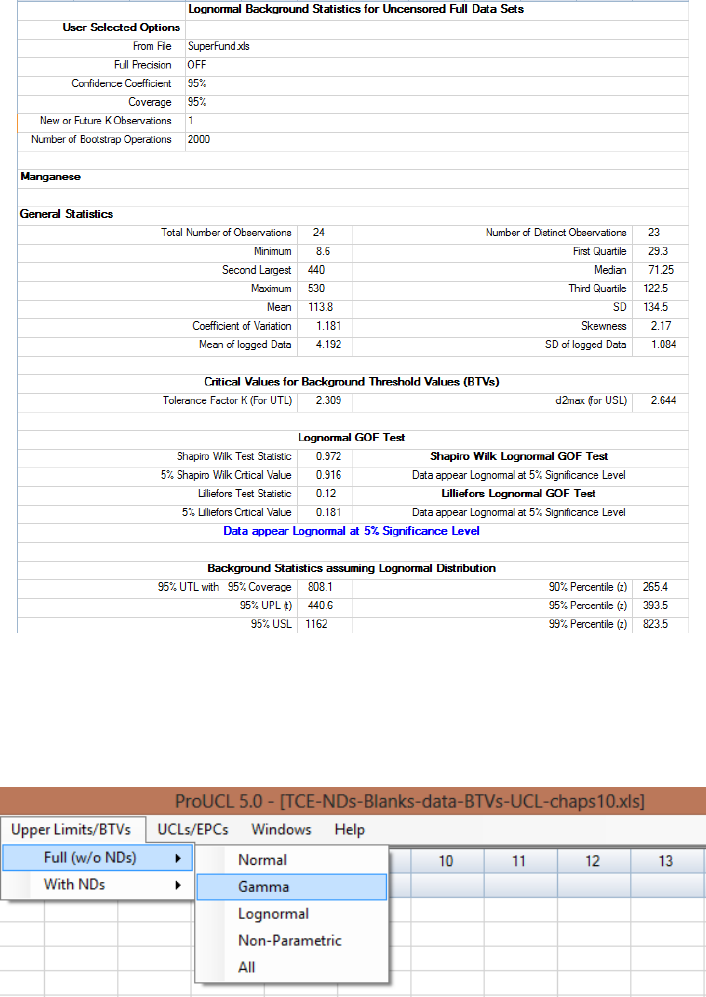
179
Manganese -Output Screen for BTV Estimates Based upon a Lognormal Distribution
(Full-Uncensored Data Set)
10.1.2 Gamma Distribution
1. Click Upper Limits/BTVs ► Full (w/o NDs) ► Gamma
2. The Select Variables screen (Chapter 3) will appear.
Select a variable(s) from the Select Variables screen.
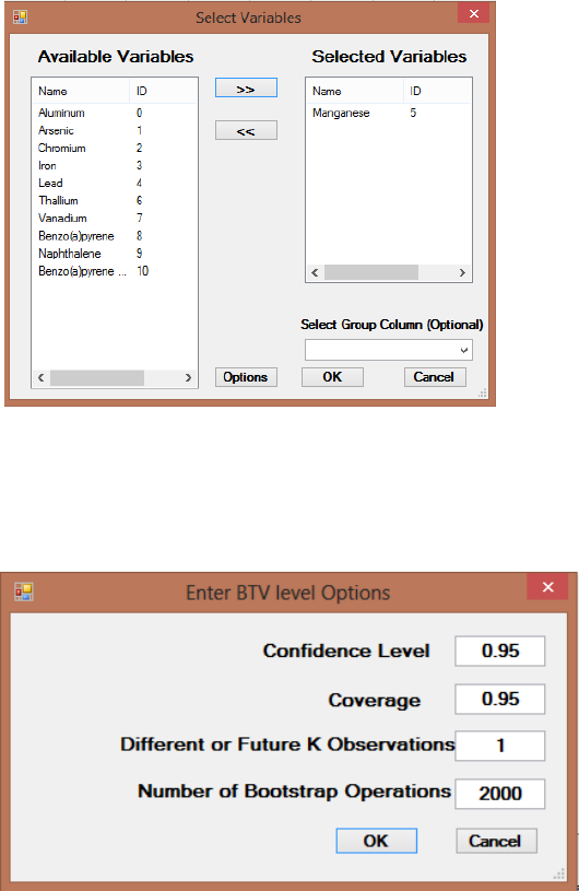
180
If needed, select a group variable by clicking the arrow below the Select Group Column
(Optional) to obtain a drop-down list of variables, and select a proper group variable.
When the Option button is clicked, the following window will be shown.
o Specify the Confidence Level; a number in the interval (0.5, 1), 0.5 inclusive. The
default choice is 0.95.
o Specify the Coverage level; a number in interval (0.0, 1). Default choice is 0.95.
o Specify the Future K. The default choice is 1.
o Specify the Number of Bootstrap Operations. The default choice is 2000.
o Click on OK button to continue or on Cancel button to cancel the option.
Click on OK to continue or on Cancel button to cancel the Upper Limits/BTVs options.
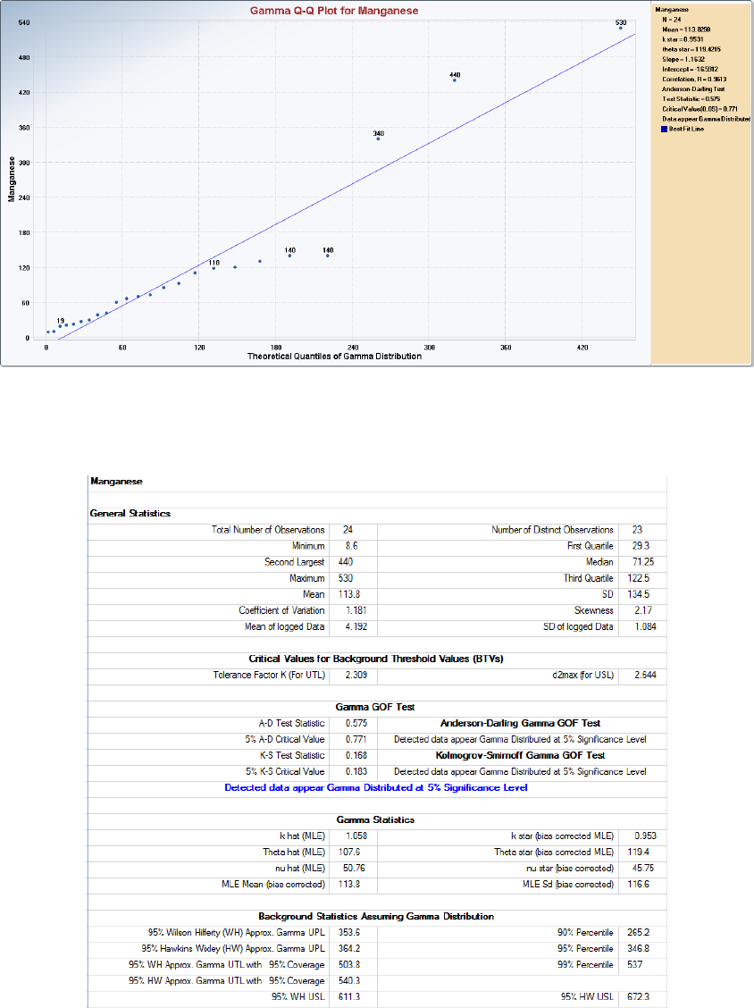
181
Example 10-1b (continued). Manganese concentrations also follow a gamma distribution. The gamma
distribution based BTV estimates are summarized in the following table generated by ProUCL 5.0. The
Gamma GOF test is shown in the following figure.
Gamma GOF Test for Manganese Data Set
Manganese - Output Screen for BTV Estimates Based Upon a Gamma Distribution
(Full-Uncensored Data Set)
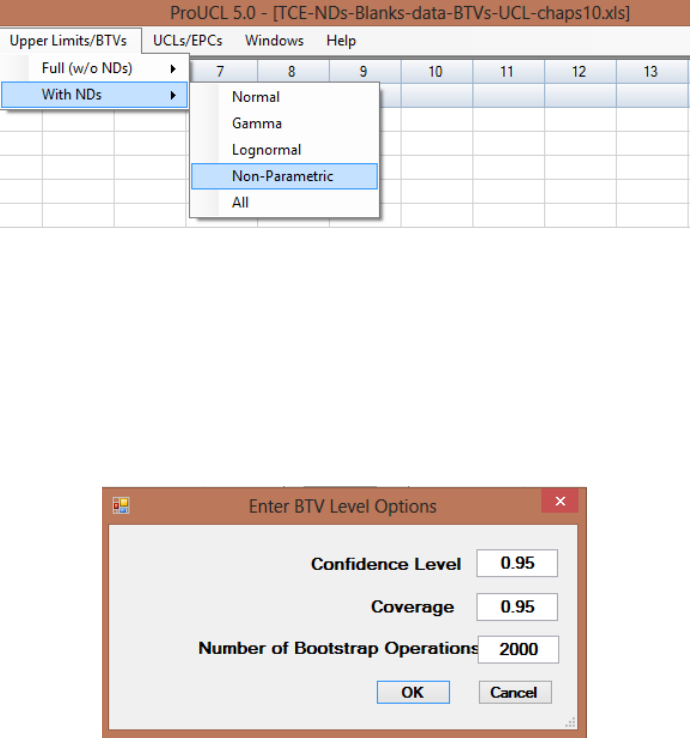
182
The mean manganese concentration is 113.8 with sd = 134.5, and the maximum value = 530. The UTL
based upon a lognormal distribution is 808.1 which is significantly higher than the largest value of 530. It
is noted that the sd of the log-transformed data is 1.084. By comparing BTV estimates computed using
lognormal and gamma distributions, it is noted that the lognormal distribution based upper limits, UTL
and UPL, are significantly higher than those based upon a gamma distribution confirming the statements
made earlier that the use of a lognormal distribution tends to yield inflated values of the upper limits used
to estimate environmental parameters (e.g., BTVs, EPCs). These upper limits are summarized as follows.
Lognormal
Gamma (WH)
Gamma (HW)
UTL95-95
808.1
504
540.3
UPL95
440.6
353.6
364.2
Mean = 113.8, Max value = 530.
10.1.3 Nonparametric Methods
1. Click Upper Limits/BTVs ► Full (w/o NDs) ► Non-Parametric
2. The Select Variables screen (Chapter 3) will appear.
Select a variable(s) from the Select Variables screen.
If needed, select a group variable by clicking the arrow below the Select Group Column
(Optional) to obtain a drop-down list of variables, and select a proper group variable.
When the Option button is clicked, the following window will be shown.
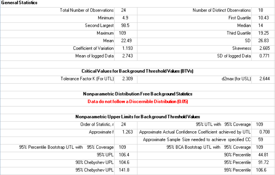
183
o Specify the Confidence Level; a number in the interval (0.5, 1), 0.5 inclusive. The
default choice is 0.95.
o Specify the Coverage level; a number in the interval (0.0, 1). Default choice is 0.95.
o Specify the Number of Bootstrap Operations. The default choice is 2000.
o Click on the OK button to continue or on the Cancel button to cancel the option.
Click OK button to continue or Cancel button to cancel the Upper Limits/BTVs options.
Example 10-2. Lead concentrations data set used in Example 1-1 does not follow a discernible
distribution. Nonparametric BTV estimates are summarized as follows. ProUCL 5.1 also outputs the
sample size needed to compute a nonparametric UTL needed to achieve the specified CC.
Lead - Output Screen for Nonparametric BTVs Estimates
(Full-Uncensored Data Set)
To compute nonparametric upper limits providing the specified coverage (e.g., 0.95), sizes of the data sets
should be fairly large (e.g., > 59). For details, consult the associated ProUCL Technical Guide. In this
example the sample size is only 24, and the confidence coefficient (CC) achieved by the nonparametric,
UTL is only 0.71 which is significantly lower than the desired CC of 0.95.
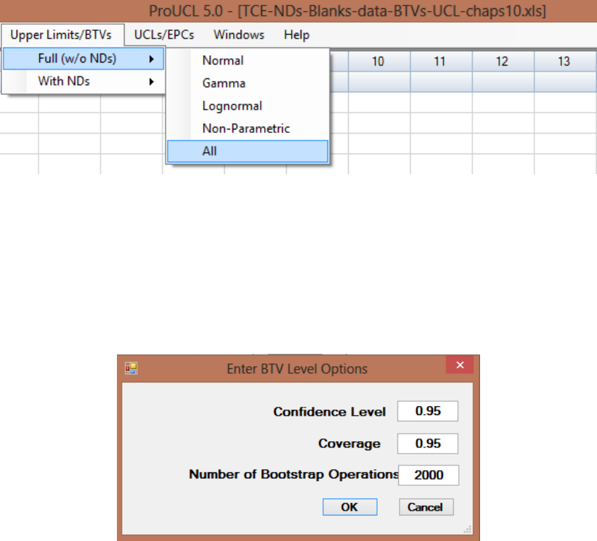
184
10.1.4 All Statistics Option
1. Click Upper Limits/BTVs ► Full (w/o NDs) ► All
2. The Select Variables screen (Chapter 3) will appear.
Select a variable(s) from the Select Variables screen.
If needed, select a group variable by clicking the arrow below the Select Group Column
(Optional) to obtain a drop-down list of variables, and select a proper group variable.
When the Option button is clicked, the following window will be shown.
o Specify the Confidence Level; a number in the interval (0.5, 1), 0.5 inclusive. The
default choice is 0.95.
o Specify the Coverage level; a number in the interval (0.0, 1). Default is 0.9.
o Specify the Future K. The default choice is 1.
o Specify the Number of Bootstrap Operations. The default choice is 2000.
o Click on OK button to continue or on Cancel button to cancel the option.
Click on OK to continue or on Cancel button to cancel the Upper Limits/BTVs options.
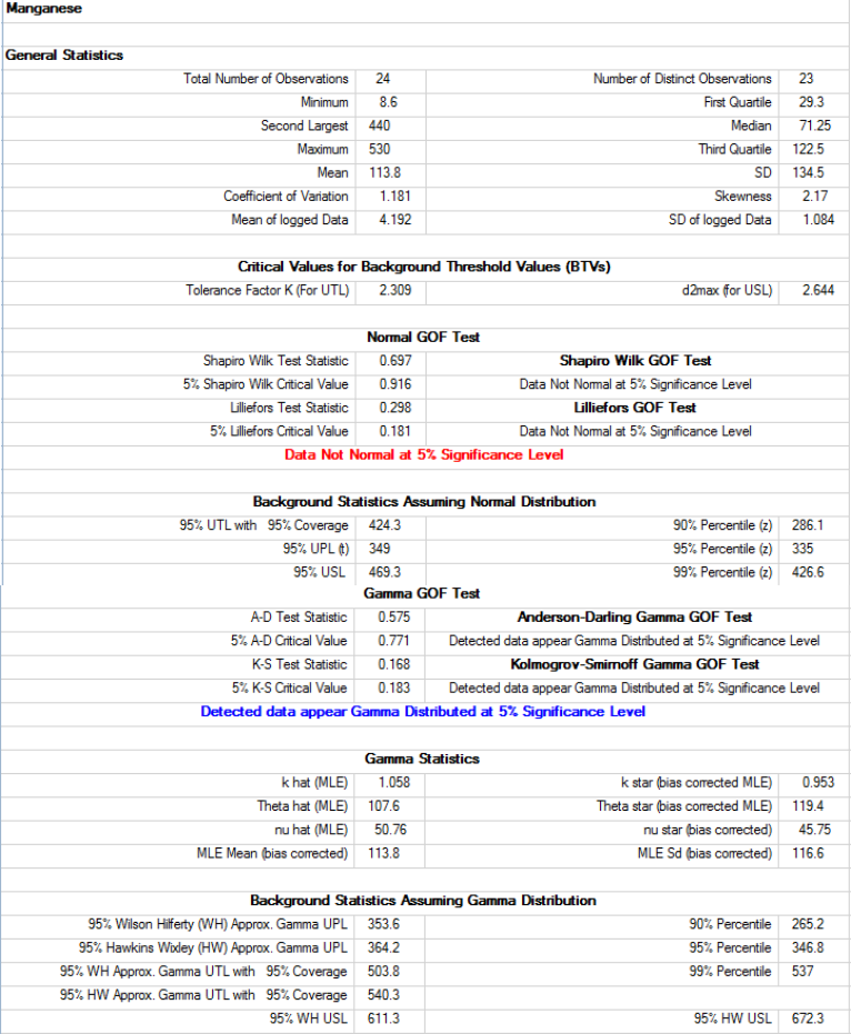
185
Example 10-1c (continued). The various BTV estimates based upon the manganese concentrations
computed using the All option of ProUCL are summarized as follows. The All option computes and
displays all available parametric and nonparametric BTV estimates. This option also informs the user
about the distribution(s) of the data set. This option is specifically useful when one has to process many
analytes (variables) without any knowledge about their probability distributions.
Manganese - Output Screen for All BTVs Estimates
(Full-Uncensored Data Set)
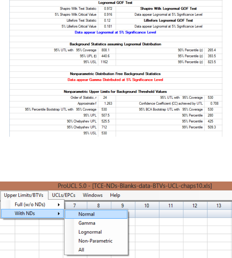
186
Manganese - Output Screen for All BTVs Estimates - Continued
(Full-Uncensored Data Set)
10.2 Background Statistics with NDs
1. Click Upper Limits/BTVs ► With NDs
2. Select the With NDs option.
To compute background statistics assuming the normal distribution, click on Normal
from the drop-down menu list.
To compute background statistics assuming the gamma distribution, click on Gamma
from the drop-down menu list.
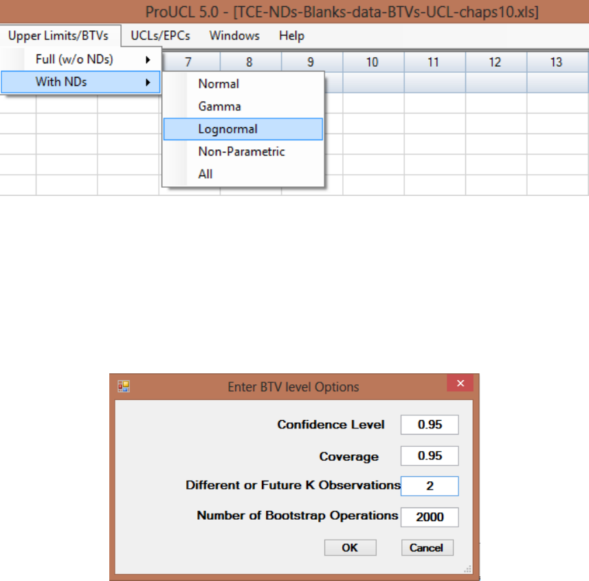
187
To compute background statistics assuming the lognormal distribution, click on
Lognormal from the drop-down menu list.
To compute background statistics using distribution-free methods, click on Non-
Parametric from the drop-down menu list.
To compute all available background statistics in ProUCL, click on the All option from
the drop-down menu list.
10.2.1 Normal or Lognormal Distribution
1. Click Upper Limits/BTVs ► With NDs ► Normal or Lognormal
2. The Select Variables screen (Chapter 3) will appear.
Select a variable(s) from the Select Variables screen.
If needed, select a group variable by clicking the arrow below the Select Group Column
(Optional) to obtain a drop-down list of variables, and select a proper group variable.
When the option button is clicked, the following window will be shown.
o Specify the Confidence Level; a number in the interval (0.5, 1), 0.5 inclusive. The
default choice is 0.95.
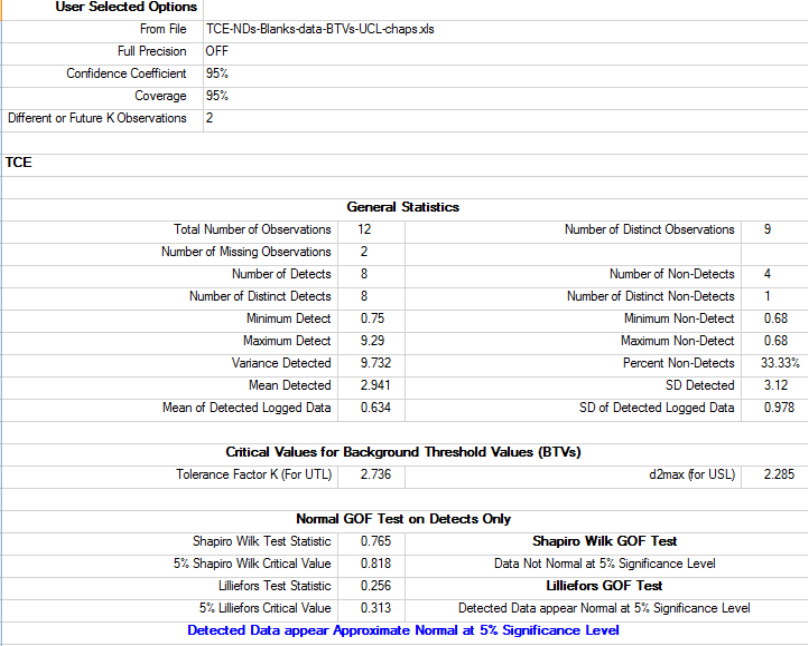
188
o Specify the Coverage level; a number in the interval (0.0, 1). Default choice is 0.95.
o Specify the Future K. The default choice is 1.
o Specify the Number of Bootstrap Operations. The default choice is 2000.
o Click on the OK button to continue or on the Cancel button to cancel the option.
Click on OK to continue or on Cancel button to cancel the Upper limits/BTVs options.
Example 10-3a. Consider a small real TCE data set of size n=12 consisting of 4 ND observations.
The detected data set of size 8 follows a normal as well as a lognormal distribution. The BTV
estimates using the LROS method, normal and lognormal distribution on KM estimates, and
nonparametric Chebyshev inequality and bootstrap methods on KM estimates are summarized in the
following two tables. It is noted that upper limits including UTL95-95 and UPL95 based upon the
robust LROS method yield much higher values than the other methods including KM estimates in
normal and lognormal equations to compute the upper limits. It is noted that the detected data also
follows a gamma distribution. The gamma distribution (of detected data) based BTV estimates are
described in the next section.
TCE - Output Screen for BTV Estimates Computed Using Normal Distribution of Detected Data
(Left-Censored Data Set with NDs)
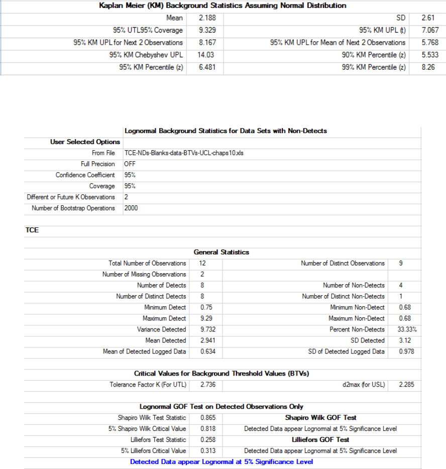
189
TCE (continued) - Output Screen for BTV Estimates Computed Using Normal Distribution of
Detected Data (Left-Censored Data Set with NDs)
Output Screen for BTV Estimates Computed Using a Lognormal Distribution of Detected Data
(Left-Censored Data Set with NDs)
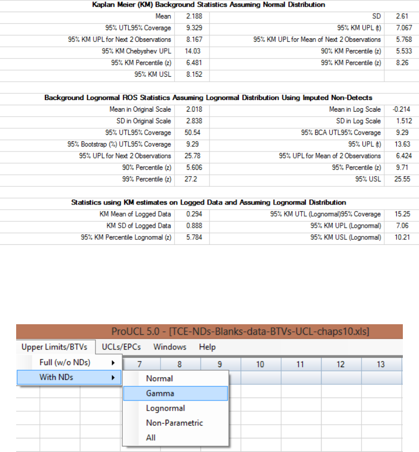
190
Continued: Output Screen for BTV Estimates Computed Using a Lognormal Distribution of
Detected Data (Left-Censored Data Set with NDs)
10.2.2 Gamma Distribution
1. Click Upper Limits/BTVs ► With NDs ► Gamma
2. The Select Variables screen (Chapter 3) will appear.
Select a variable(s) from the Select Variables screen.
If needed, select a group variable by clicking the arrow below the Select Group Column
(Optional) to obtain a drop-down list of variables, and select a proper group variable.
When the Option button is clicked, the following window will be shown.
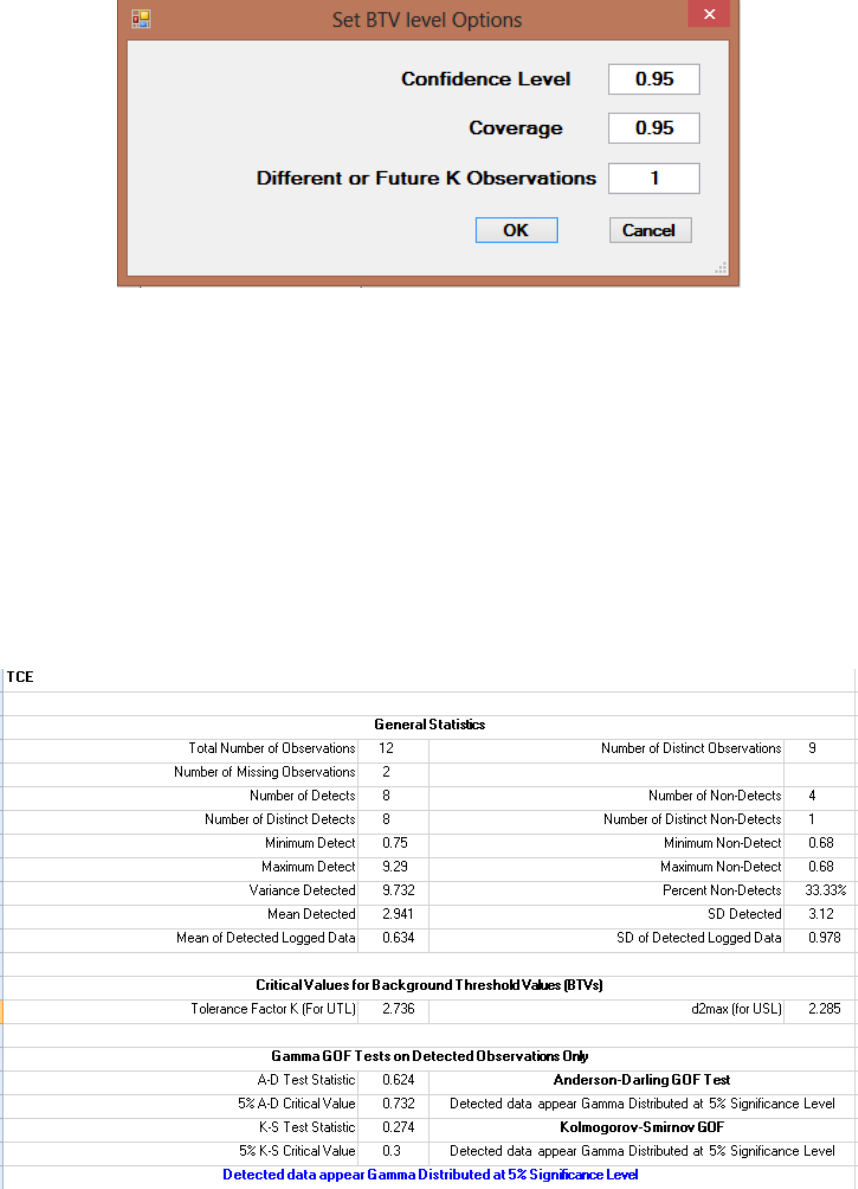
191
o Specify the Confidence Level; a number in the interval (0.5, 1), 0.5 inclusive. The
default choice is 0.95.
o Specify the Coverage level; a number in the interval (0.0, 1). Default choice is 0.95.
o Click on the OK button to continue or on the Cancel button to cancel option.
Click on OK to continue or on Cancel button to cancel the Upper Limits/BTVs options.
Example 10-3b (continued). It is noted that the detected TCE data considered in Example 10-3 also
follows a gamma distribution. The gamma distribution based upper limits are summarized as follows.
TCE - Output Screen for BTV Estimates Computed Using Gamma Distribution of Detected Data
(Left-Censored Data Set with NDs)
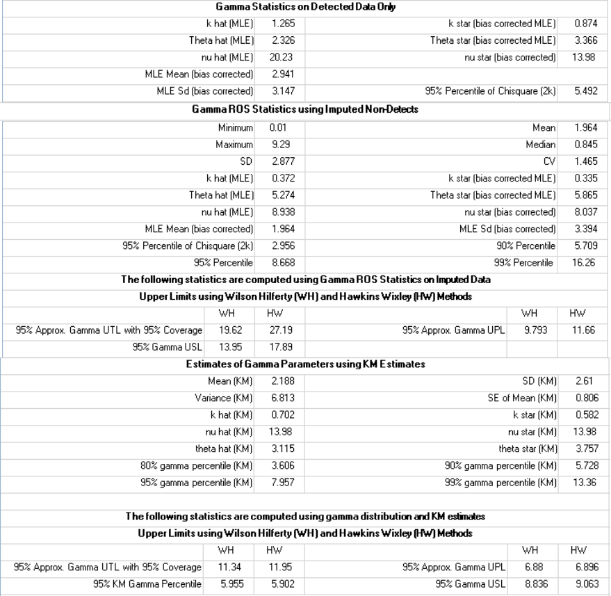
192
TCE (continued) - Output Screen for BTV Estimates Computed Using Gamma Distribution of
Detected Data (Left-Censored Data Set with NDs)
The detected data set does not follow a normal distribution based upon the S-W test, but follows a normal
distribution based upon the Lilliefors test. Since the detected data set is of small size (=8), the normal
GOF conclusion is suspect. The detected data follow a gamma distribution. There are several NDs
reported with a low detection limit of 0.68, therefore, GROS method may yield infeasible negative
imputed values. Therefore, the use of a gamma distribution on KM estimates is preferred for computing
the BTV estimates. The gamma KM UTL95-95 (HW) =11.34, and gamma KM UTL95-95 (WH) = 11.95.
Any one of these two limits can be used to estimate the BTV.
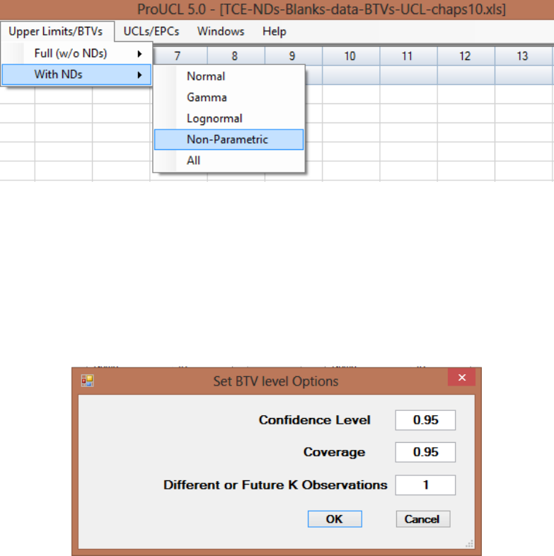
193
10.2.3 Nonparametric Methods (with NDs)
1. Click Upper Limits/BTVs► With NDs ► Non-Parametric
2. The Select Variables screen (Chapter 3) will appear.
Select a variable(s) from the Select Variables screen.
If needed, select a group variable by clicking the arrow below the Select Group Column
(Optional) to obtain a drop-down list of variables, and select a proper group variable.
When the Option button is clicked, the following window will be shown.
o Specify the Confidence Level; a number in the interval (0.5, 1), 0.5 inclusive. The
default choice is 0.95.
o Specify the Coverage level; a number in interval (0.0, 1). Default choice is 0.95.
o Click on the OK button to continue or on the Cancel button to cancel the option.
Click on OK to continue or on Cancel button to cancel the Upper Limit/BTVs option.
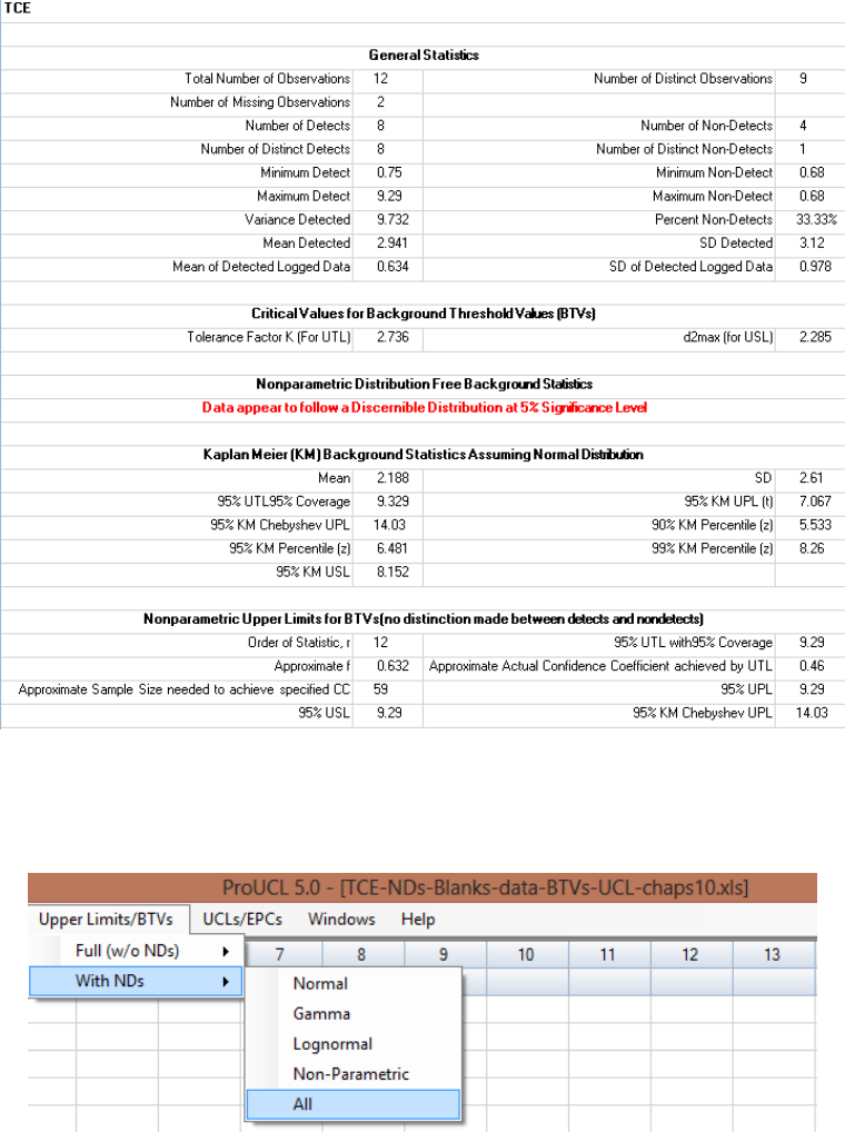
194
Example 10-3c (continued). The nonparametric upper limits based the TCE data considered in Example
10-3 are summarized in the following table.
TCE - Output Screen for Nonparametric BTV Estimates
(Left-Censored Data Set with NDs)
10.2.4 All Statistics Option
1. Click Upper Limits/BTVs ► With NDs ► All
2. The Select Variables screen (Chapter 3) will appear.
Select a variable(s) from the Select Variables screen.
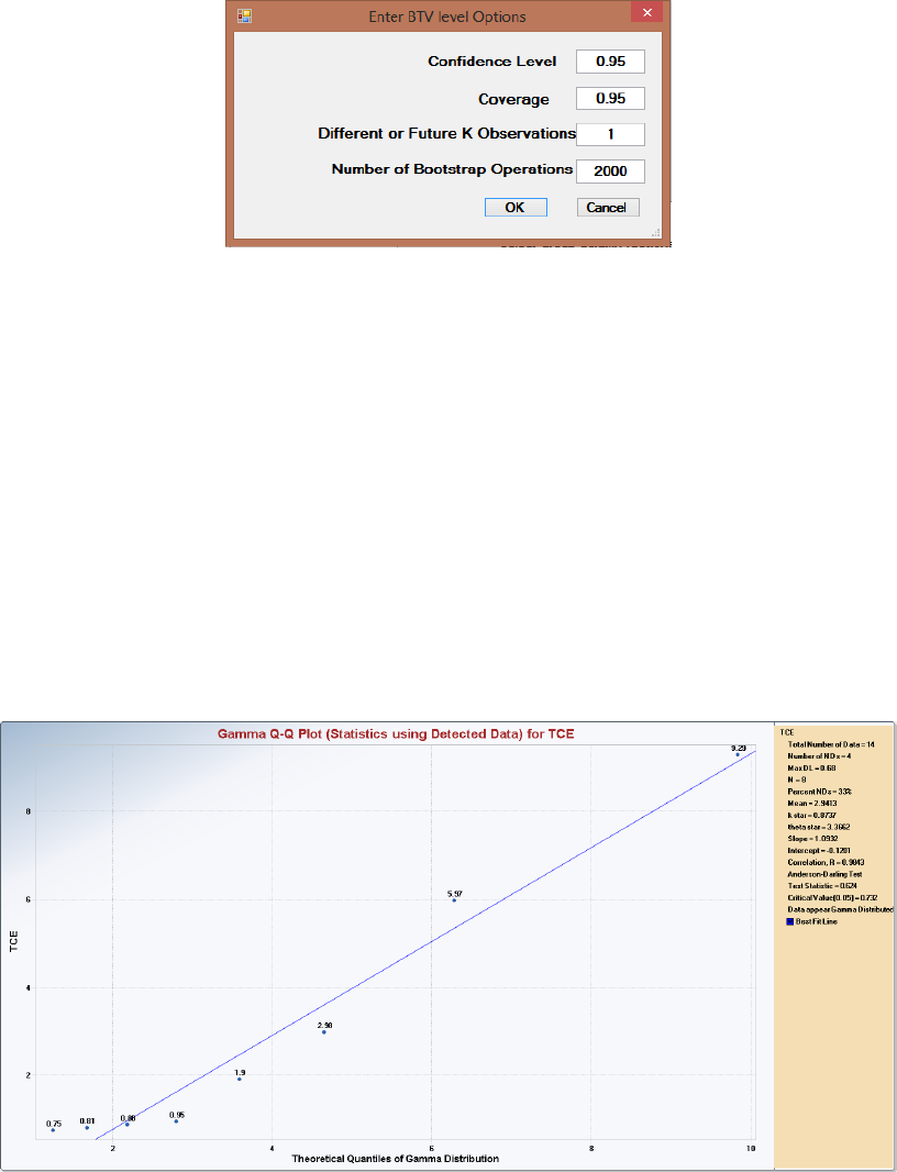
195
If needed, select a group variable by clicking the arrow below the Select Group Column
(Optional) to obtain a drop-down list of variables, and select a proper group variable.
When the Option button is clicked, the following window will be shown.
o Specify the Confidence Level; a number in the interval (0.5, 1), 0.5 inclusive. The
default choice is 0.95.
o Specify the Coverage level; a number in the interval (0.0, 1). Default choice is 0.95.
o Specify the Future K. The default choice is 1.
o Click on the OK button to continue or on the Cancel button to cancel the option.
Click on OK to continue or on Cancel button to cancel the Upper Limits/BTVs option.
Example 10-3d (continued). BTV estimates using the All option for the TCE data are summarized as
follows. The detected data set is of small size (n=8) and follows a gamma distribution. The gamma GOF
Q-Q plot based upon detected data is shown in the following figure. The relevant statistics have been
high-lighted in the output table provided after the gamma GOF Q-Q plot.
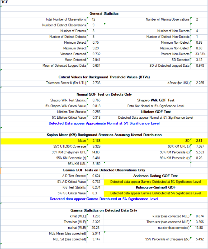
196
TCE - Output Screen for All BTV Estimates (Left-Censored Data Set with NDs)
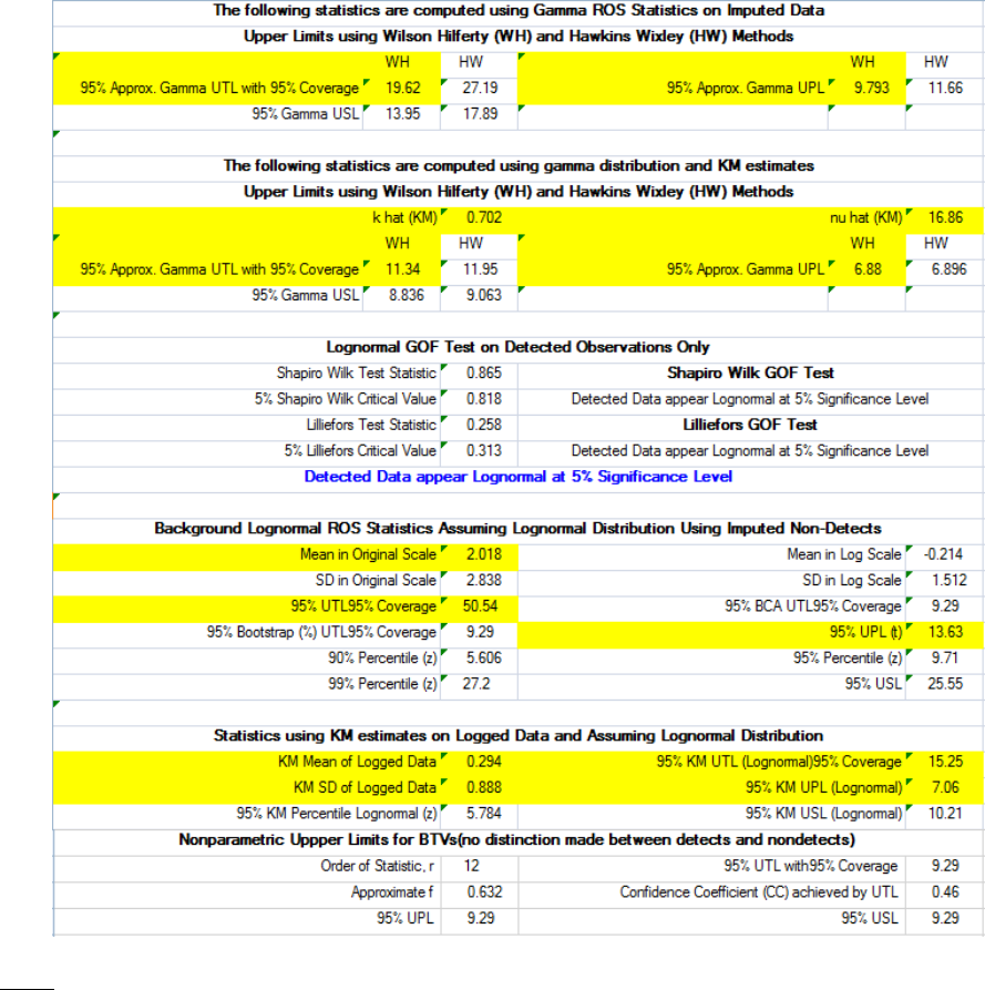
197
TCE (continued) - Output Screen for All BTV Estimates (Left-Censored Data Set with NDs)
Note: Even though the data set failed the Shapiro-Wilk test of normality, based upon Lilliefors test it was
concluded that the data set follows a normal distribution. Therefore, instead of saying that the data set
does not follow a normal distribution, ProUCL outputs that the data set follows an approximate normal
distribution. In practice the two tests can lead to different conclusions, especially when the data set is of
small size. In such instances, the user may want to select a distribution (if any) passing both of the GOF
tests. It is also suggested that the user supplements test results with graphical displays to derive the final
conclusion.
As noted, detected data follow a gamma as well as a lognormal distribution. The various upper limits
using Gamma ROS and Lognormal ROS methods and Gamma and Lognormal distribution on KM
estimates are summarized as follows.

198
Summary of Upper Limits Computed using Gamma and Lognormal Distribution of Detected Data
Sample Size = 12, No. of NDs = 4, % NDs = 33.33, Max Detect = 9.29
Upper Limits
Gamma Distribution
Lognormal Distribution
Result
Reference/
Method of Calculation
Result
Reference/
Method of Calculation
Mean (KM)
2.188
--
0.29
Logged
Mean (ROS)
1.964
--
2.018
--
UPL95 (ROS)
9.79
WH- ProUCL(ROS)
13.63
Helsel (2012), EPA (2009)-
LROS
UTL95-95 (ROS)
19.62
WH- ProUCL(ROS)
50.54
Helsel (2012), EPA (2009)-
LROS
UPL95 (KM)
6.88
WH - ProUCL (KM-
Gamma)
7.06
KM-Lognormal EPA (2009)
UTL95-95 (KM)
11.34
WH - ProUCL (KM-
Gamma)
15.25
KM- Lognormal EPA(2009)
Note: All computations have been performed using the ProUCL software. In the above table, methods
proposed/described in the literature have been cited in the Reference Method of Calculation column. The
statistics summarized above demonstrate the merits of using the gamma distribution based upper limits to
estimate decision parameters (BTVs) of interest. These results summarized in the above tables suggest
that the use of a gamma distribution cannot be dismissed just because it is easier to use a lognormal
distribution to model skewed data sets as stated by some practitioners.
199

200
Chapter 11
Computing Upper Confidence Limits (UCLs) of Mean Based Upon
Full-Uncensored Data Sets and Left-Censored Data Sets with
Nondetects
Several parametric and nonparametric UCL methods for full-uncensored and left-censored data sets
consisting of ND observations with multiple DLs are available in ProUCL 5.1. Methods such as the
Kaplan-Meier (KM) and regression on order statistics (ROS) methods incorporated in ProUCL can handle
multiple detection limits. For details regarding the goodness-of-fit tests and UCL computation methods
available in ProUCL, consult the ProUCL Technical Guides, Singh, Singh, and Engelhardt (1997); Singh,
Singh, and Iaci (2002); and Singh, Maichle, and Lee (2006).
In ProUCL 5.0/ProUCL 5.1, two choices are available for computing UCL statistics:
Full (w/o NDs): Computes UCLs for full-uncensored data sets without any nondetects.
With NDs: Computes UCLs for data sets consisting of ND observations with multiple DLs or
reporting limits (RLs).
For full data sets without NDs and also for data sets with NDs, the following options and
choices are available to compute UCLs of the population mean.
o The user specifies a confidence level; a number in the interval (0.5, 1), 0.5 inclusive. The
default choice is 0.95.
o The program computes several nonparametric UCLs using the CLT, adjusted CLT,
Chebyshev inequality, jackknife, and bootstrap re-sampling methods.
o For the bootstrap method, the user can select the number of bootstrap runs (re-samples).
The default choice for the number of bootstrap runs is 2000.
o The user is responsible for selecting an appropriate choice for the data distribution:
normal, gamma, lognormal, or nonparametric. It is desirable that user determines data
distribution using the Goodness-of-Fit test option prior to using the UCL option. The
UCL output sheet also informs the user if data are normal, gamma, lognormal, or a non-
discernible distribution. Program computes statistics depending on the user selection.
o For data sets, which are not normal, one may try the gamma UCL next. The program will
offer you advice if you chose the wrong UCL option.
o For data sets, which are neither normal nor gamma, one may try the lognormal UCL.
The program will offer you advice if you chose the wrong UCL option.

201
o Data sets that are not normal, gamma, or lognormal are classified as distribution-free
nonparametric data sets. The user may use nonparametric UCL option for such data sets.
The program will offer you advice if you chose the wrong UCL option.
o The program also provides the All option. By selecting this option, ProUCL outputs most
of the relevant UCLs available in ProUCL. The program informs the user about the
distribution of the underlying data set, and offers advice regarding the use of an
appropriate UCL.
For lognormal data sets, ProUCL can compute 90%, 95%, 97.5%, and 99% Land’s
statistic-based H-UCL of the mean. For all other methods, ProUCL can compute a UCL
for any confidence coefficient (CC) in the interval (0.5, 1.0), 0.5 inclusive. If you have
selected a distribution, then ProUCL will provide a recommended UCL method for 0.95,
confidence level. Even though ProUCL can compute UCLs for any confidence
coefficient level in the interval (0.5, 1.0), the recommendations are provided only for
95% UCL; as EPC term is estimated by a 95% UCL of the mean.
Notes: Like all other methods, it is recommended that the user identify a few low probability (coming
from extreme tails) outlying observations that may be present in the data set. Outliers distort statistics of
interest including summary statistics, data distributions, test statistics, UCLs and BTVs. Decisions based
upon distorted statistics may be misleading and incorrect. The objective is to compute decision statistics
based upon the majority of the data set representing the main dominant population. The project team
should decide about the disposition (to include or not to include) of outliers before computing estimates
of EPCs and BTVs. To determine the influence of outliers on UCLs and background statistics, the project
team may want to compute statistics twice: once using the data set with outliers, and once using the data
set without outliers.
Note on Computing Lower Confidence Limits (LCLs) of the Mean: In several environmental
applications, one needs to compute a LCL of the population mean. At present, ProUCL does not directly
compute LCLs of mean. It should be pointed out that for data sets with and without NDs, except for the
bootstrap methods, gamma distribution (e.g., samples of sizes <50), and H-statistic based LCL of mean,
the same critical value (e.g., normal z value, Chebyshev critical value, or t-critical value) are used to
compute a LCL of mean as used in the computation of the UCL of mean. Specifically, to compute a LCL,
the '+' sign used in the computation of the corresponding UCL needs to be replaced by the '-' sign in the
equation used to compute that UCL (excluding gamma, lognormal H-statistic, and bootstrap methods).
For specific details, the user may want to consult a statistician. For data sets without nondetect
observations, the user may want to use the Scout 2008 software package (EPA 2009c) to directly compute
the various parametric and nonparametric LCLs of mean.
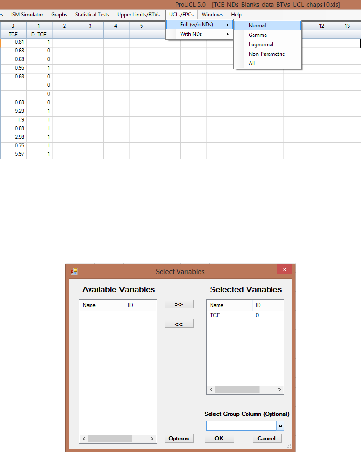
202
11.1 UCLs for Full (w/o NDs) Data Sets
11.1.1 Normal Distribution (Full Data Sets without NDs)
1. Click UCLs/EPCs ► Full (w/o NDs) ► Normal
2. The Select Variables screen (Chapter 3) will appear.
Select a variable(s) from the Select Variables screen.
If needed, select a group variable by clicking the arrow below the Select Group Column
(Optional) to obtain a drop-down list of available variables to select a group variable.
When the Option button is clicked, the following window will be shown.
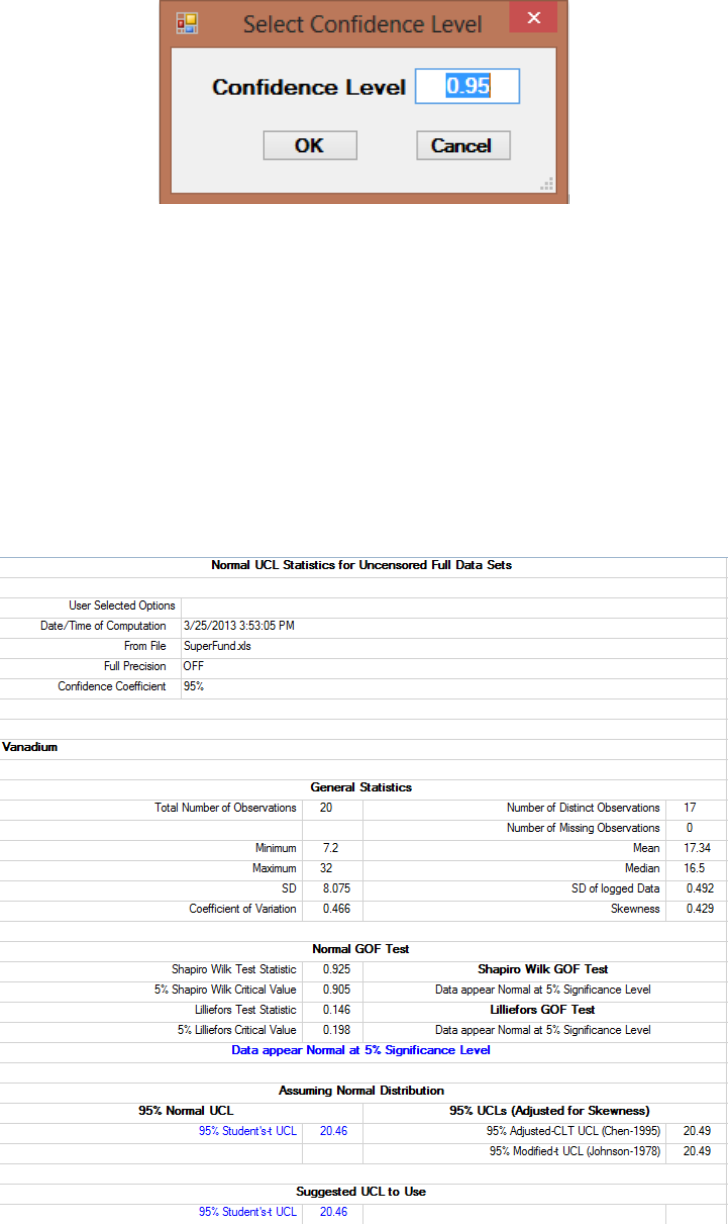
203
o Specify the Confidence Level; a number in the interval (0.5, 1), 0.5 inclusive. The
default choice is 0.95.
o Click on OK button to continue or on Cancel button to cancel the option.
Click on OK to continue or on Cancel to cancel the UCL computation option.
Example 11-1. Consider the data used in Example 1-1 collected from a Superfund site; vanadium
concentrations follow a normal distribution. The normal distribution based 95% UCLs of mean are
summarized in the following table.
Vanadium - Output Screen for Normal Distribution (Full Data w/o NDs)
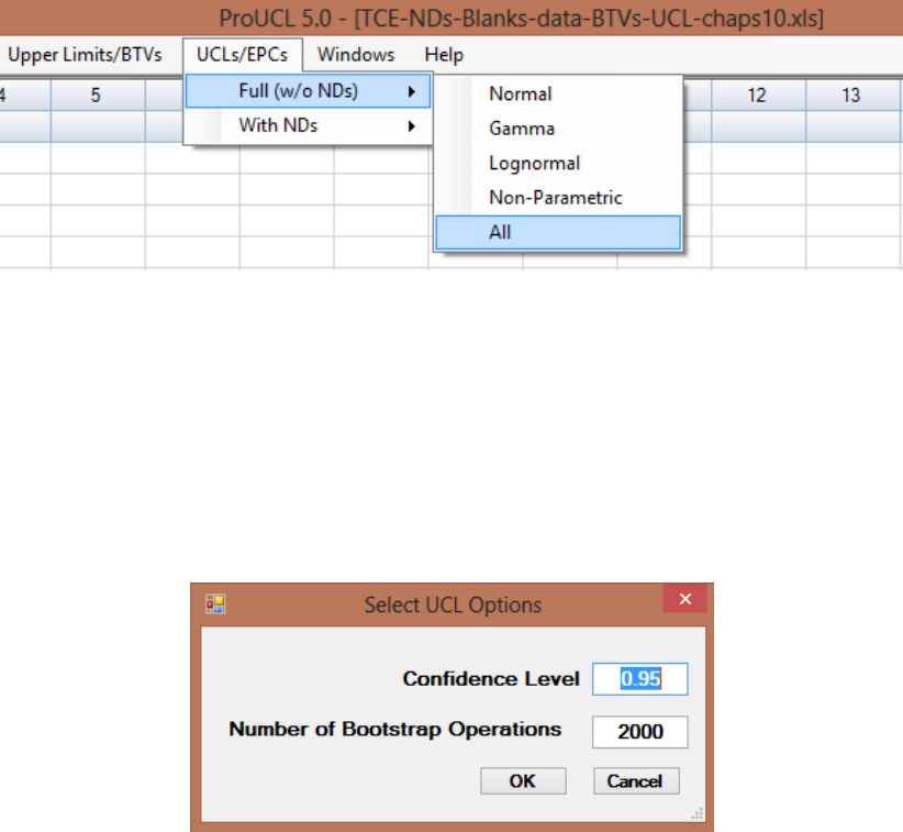
204
11.1.2 Gamma, Lognormal, Nonparametric, All Statistics Option (Full Data without NDs)
1. Click UCLs/EPCs ► Full (w/o NDs) ► Gamma, Lognormal, Non-Parametric, or All
2. The Select Variables screen (Chapter 3) will appear.
Select a variable(s) from the Select Variables screen.
If needed, select a group variable by clicking the arrow below the Select Group Column
(Optional) to obtain a drop-down list of available variables, and select a proper group
variable.
When the Option button is clicked, the following window will be shown.
o Specify the Confidence Level; a number in the interval [0.5, 1), 0.5 inclusive.
o Specify the Number of Bootstrap Operations (runs). Default choice is 2000.
o Click on OK button to continue or on Cancel button to cancel the UCLs option.
Click on OK to continue or on Cancel to cancel the selected UCL computation option.
Example 11-2: This skewed data set of size n=25 with mean=44.09 was used in Chapter 2 of the
Technical Guide. The data follows a lognormal and a gamma distribution. The data are: 0.3489, 0.8526,
2.5445, 2.5602, 3.3706, 4.8911, 5.0930, 5.6408, 7.0407, 14.1715, 15.2608, 17.6214, 18.7690, 23.6804,
25.0461, 31.7720, 60.7066, 67.0926, 72.6243, 78.8357, 80.0867, 113.0230, 117.0360, 164.3302, and
169.8303. UCLs based upon Gamma, Lognormal, Non-parametric, and All options are summarized in
the following tables.
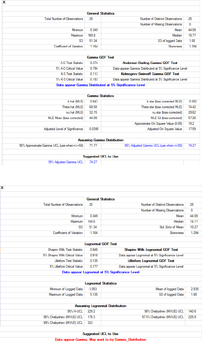
205
Output Screen for Gamma Distribution Based UCLs (Full [w/o NDs])
Output Screen for Lognormal Distribution Based UCLs (Full [w/o NDs])
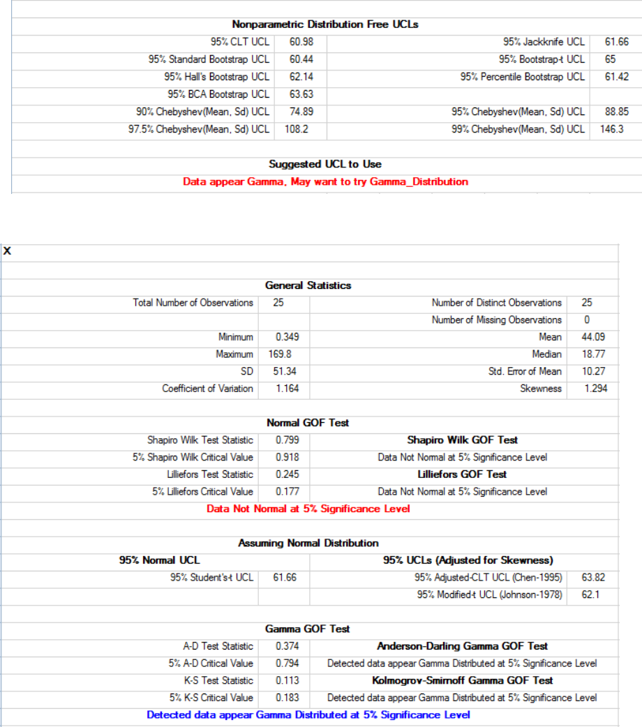
206
Output Screen for Nonparametric UCLs (Full [w/o NDs])
Output Screen for All Statistics Option (Full [w/o NDs])
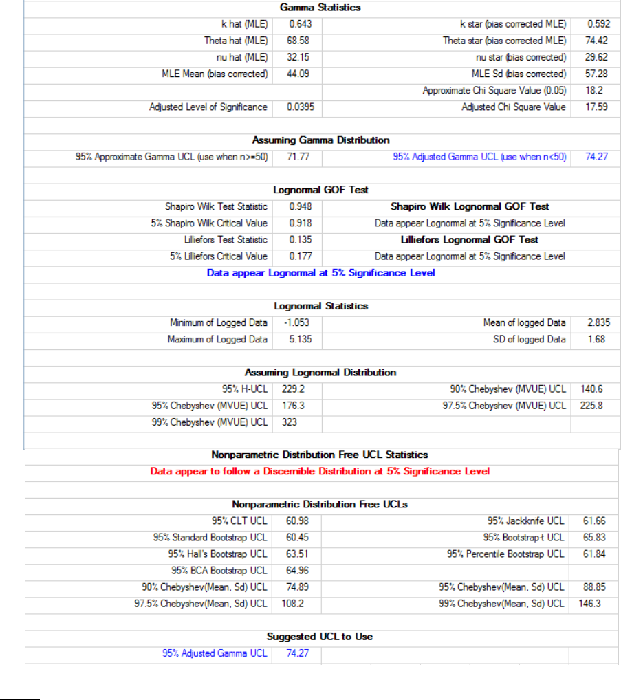
207
Continued: Output Screen for All Statistics Option (Full [w/o NDs])
Notes: Once again, the statistics summarized above demonstrate the merits of using the gamma
distribution based UCL of mean to estimate EPCs. The use of a lognormal distribution tends to yield
unrealistic UCLs without practical merit (e.g., Lognormal UCL = 229.2 and the maximum = 169.8 in the
above example). The results summarized in the above tables suggest that the use of a gamma distribution
(when a data set follows a gamma distribution) cannot be dismissed just because it is easier (Helsel and
Gilroy 2012) to use a lognormal distribution to model skewed data sets.
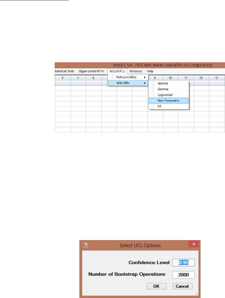
208
Number of valid samples represents the total number of samples minus (-) the missing values (if any).
The number of unique or distinct samples simply represents number of distinct observations. The
information about the number of distinct values is useful when using bootstrap methods. Specifically, it is
not desirable to use bootstrap methods on data sets with only a few distinct values.
11.2 UCL for Left-Censored Data Sets with NDs
1. Click UCLs/EPCs ► With NDs
2. Choose the Normal, Gamma, Lognormal, Non-Parametric, or All option.
3. The Select Variables screen (Chapter 3) will appear.
Select a variable(s) from the Select Variables screen.
If needed, select a group variable by clicking the arrow below the Select Group Column
(Optional) to obtain a drop-down list of available variables, and select a proper group
variable. The selection of this option will compute the relevant statistics separately for
each group that may be present in the data set.
When the Option button is clicked, the following window will be shown.
o Specify the Confidence Level; a number in the interval (0.5, 1), 0.5 inclusive. The
default choice is 0.95.
o Specify the Number of Bootstrap Operations (runs). Default choice is 2000.
o Click on OK button to continue or on Cancel button to cancel the UCLs option.
Click on OK to continue or on Cancel to cancel the selected UCL computation option.
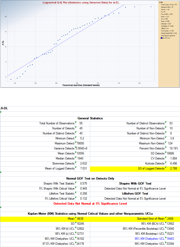
209
Example 11-3. This real data set of size n=55 with 18.8% NDs (=10) is also used in Chapters 4 and 5 of
the ProUCL Technical Guide. The minimum detected value is 5.2 and the largest detected value is 79000,
sd of detected logged data is 2.79 suggesting that the data set is highly skewed. The detected data follow a
gamma as well as a lognormal distribution. It is noted that GROS data set with imputed values follows a
gamma distribution and LROS data set with imputed values follows a lognormal distribution (results not
included). The lognormal Q-Q plot based upon detected data is shown in the following figure. The
various UCL output sheets: normal, nonparametric, gamma, and lognormal generated by ProUCL are
summarized in tables following the lognormal Q-Q plot on detected data. The main results have been
high-lighted in the output screen provided after the lognormal GOF Q-Q plot.
Output Screen for UCLs based upon Normal, Lognormal, and Gamma Distributions (of Detects)
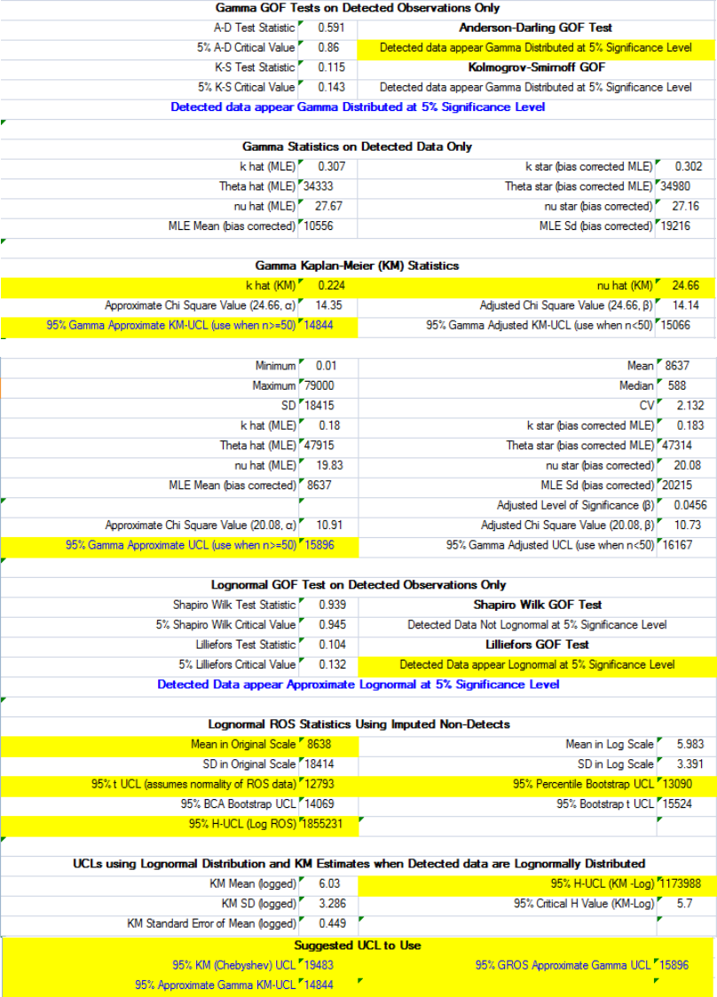
210
Continued: Output Screen for UCLs based upon Normal, Lognormal, and Gamma Distributions
(of Detects)
GROS Statistics using imputed NDs

211
Detected data follow a gamma as well as a lognormal distribution. The various upper limits using Gamma
ROS and Lognormal ROS methods and Gamma and Lognormal distribution on KM estimates are
summarized in the following table.
Upper Confidence Limits Computed using Gamma and Lognormal Distributions of Detected Data
Sample Size = 55, No. of NDs=10, % NDs = 18.18%
Upper Limits
Gamma Distribution
Lognormal Distribution
Result
Reference/
Method of Calculation
Result
Reference/
Method of Calculation
Min (detects)
5.2
--
1.65
Logged
Max (detects)
79000
--
11.277
Logged
Mean (KM)
8638
--
6.3
Logged
Mean (ROS)
8637
--
8638
--
UCL95 (ROS)
15896
ProUCL 5.0 -GROS
14863
bootstrap-t on LROS,
ProUCL 5.0
12918
percentile bootstrap on
LROS, Helsel(2012)
UCL (KM)
14844
ProUCL 5.0 - KM-Gamma
1173988
H-UCL, KM mean and
sd on logged data, EPA
(2009)
All computations have been performed using the ProUCL software. In the above table, methods
proposed/described in the literature have been cited in the Reference Method of Calculation column.
The results summarized in the above table re-iterate that the use of a gamma distribution cannot be
dismissed just because it is easier to use a lognormal distribution to model skewed data sets. These
results also demonstrate that for skewed data sets, one should use bootstrap methods which adjust for
data skewness (e.g., bootstrap- t method) rather than using percentile bootstrap method.

212
Chapter 12
Sample Sizes Based Upon User Specified Data Quality Objectives
(DQOs) and Power Assessment
One of the most frequent problems in the application of statistical theory to practical applications,
including environmental projects, is to determine the minimum number of samples needed for sampling
of reference/background areas and survey units (e.g., potentially impacted site areas, areas of concern,
decision units) to make cost-effective and defensible decisions about the population parameters based
upon the sampled discrete data. The sample size determination formulae for estimation of the population
mean (or some other parameters) depend upon certain decision parameters including the confidence
coefficient, (1-α) and the specified error margin (difference), Δ from the unknown true population mean,
µ. Similarly, for hypotheses testing approaches, sample size determination formulae depend upon pre-
specified values of the decision parameters selected while describing the data quality objectives (DQOs)
associated with an environmental project. The decision parameters associated with hypotheses testing
approaches include Type I (false positive error rate, α) and Type II (false negative error rate, β=1-power)
error rates; and the allowable width, Δ of the gray region. For values of the parameter of interest (e.g.,
mean, proportion) lying in the gray region, the consequences of committing the two types of errors
described above are not significant from both human health and cost-effectiveness point of view.
Note: Initially, the Sample Sizes module was incorporated in ProUCL 4.0/ProUCL 4.1. Not many
changes have been made in ProUCL 5.0/ProUCL 5.1 except those described below. Therefore, many
screenshots generated using an earlier 2010 version of ProUCL have been used in the examples described
in this chapter.
Both parametric (assuming normality) and nonparametric (distribution free) sample size determination
formulae as described in guidance documents (MARSSIM 2000, EPA 2002c and 2006a) have been
incorporated in the ProUCL software. Specifically, the DQOs Based Sample Sizes module of ProUCL
can be used to determine sample sizes to estimate the mean, perform parametric and nonparametric
single-sample and two-sample hypothesis tests, and apply acceptance sampling approaches to address
project needs of the various CERCLA and RCRA site projects. The details can be found in Chapter 8 of
the ProUCL Technical Guide and in EPA guidance documents (EPA 2006a, 2006b).
New in ProUCL 5.0/ProUCL 5.1: The Sample size module in ProUCL 5.0/ProUCL 5.1 can be used at
two different stages of a project. Most of the sample size formulae require some estimate of the
population standard deviation (variability). Depending upon the project stage, a standard deviation: 1)
represents a preliminary estimate of the population (e.g., study area) variability needed to compute the
minimum sample size during the planning and design stage; or 2) represents the sample standard
deviation computed using the data collected without considering DQOs process which is used to assess
the power of the test based upon the collected data. During the power assessment stage, if the computed
sample size is larger than the size of already collected data set, it can be inferred that the size of the
collected data set is not large enough to achieve the desired power. The formulae to compute the sample
sizes during the planning stage and after performing a statistical test are the same except that the estimates
of standard deviations are computed/estimated differently.
Planning stage before collecting data: Sample size formulae are commonly used during the planning stage
of a project to determine the minimum sample sizes needed to address project objectives (estimation,
hypothesis testing) with specified values of the decision parameters (e.g., Type I and II errors, width of
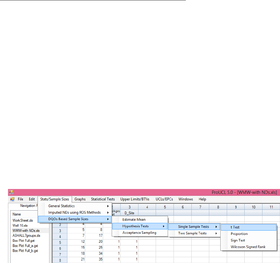
213
gray region). During the planning stage, since the data are not collected a priori, a preliminary rough
estimate of the population standard deviation (to be expected in sampled data) is obtained from other
similar sites, pilot studies, or expert opinions. An estimate of the expected standard deviation along with
the specified values of the other decision parameters are used to compute the minimum sample sizes
needed to address the project objectives during the sampling planning stage; the project team is expected
to collect the number of samples thus obtained. The detailed discussion of the sample size determination
approaches during the planning stage can be found in MARSSIM 2000 and U.S. EPA 2006a.
Power assessment stage after performing a statistical method: Often, in practice, environmental
samples/data sets are collected without taking the DQOs process into consideration. Under this scenario,
the project team performs statistical tests on the available already collected data set. However, once a
statistical test (e.g., WMW test) has been performed, the project team can assess the power associated
with the test in retrospect. That is for specified DQOs and decision errors (Type I error and power of the
test [=1-Type II error]), using the sample standard deviation computed based upon the already collected
data, the minimum sample size needed to perform the test for specified values of the decision parameters
is computed.
If the computed sample size obtained using the sample variance is less than the size of the already
collected data set used to perform the test, it may be determined that the power of the test has
been achieved. However, if the sample size of the collected data is less than the minimum sample
size computed in retrospect, the user may want to collect additional samples to assure that the test
achieves the desired power.
It should be pointed out that there could be differences in the sample sizes computed in two
different stages due to the differences in the values of the estimated variability. Specifically, the
preliminary estimate of the variance computed using information from similar sites could be
significantly different from the variance computed using the available data already collected from
the study area under investigation which will yield different values of the sample size.
Sample size determination methods in ProUCL can be used for both stages. The only difference will be in
the input value of the standard deviation/variance. It is user's responsibility to input a correct value for
the standard deviation during the two stages.
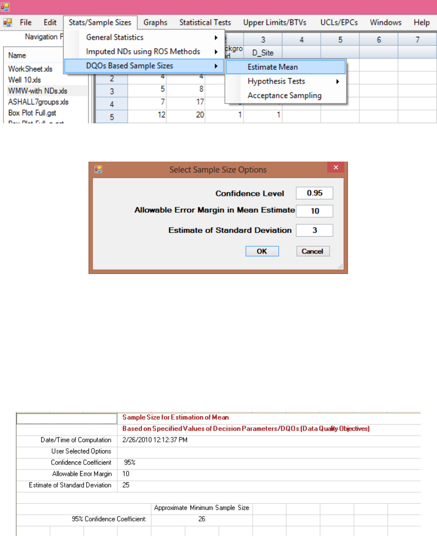
214
12.1 Estimation of Mean
1. Click Stats/Sample Sizes► DQOs Based Sample Sizes ► Estimate Mean
2. The following options window is shown.
Specify the Confidence Coefficient. Default is 0.95.
Specify the Estimate of standard deviation. Default is 3.
Specify the Allowable Error Margin in Mean Estimate. Default is 10.
Click on OK button to continue or on Cancel button to cancel the options.
Output Screen for Sample sizes for Estimation of Mean (CC = 95%, sd = 25, Error Margin = 10)
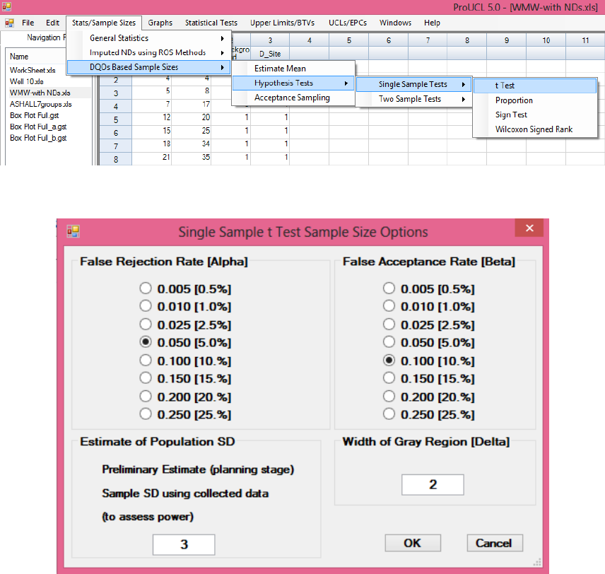
215
12.2 Sample Sizes for Single-Sample Hypothesis Tests
12.2.1 Sample Size for Single-Sample t-Test
1. Click DQOs Based Sample Sizes ► Hypothesis Tests► Single Sample Tests► t Test
The following options window is shown.
Specify the False Rejection Rate (Alpha, α). Default is 0.05.
Specify the False Acceptance Rate (Beta, β). Default is 0.1.
Specify the Estimate of standard deviation. Default is 3.
Specify the Width of the Gray Region (Delta, Δ). Default is 2.
Click on OK button to continue or on Cancel button to cancel the options.
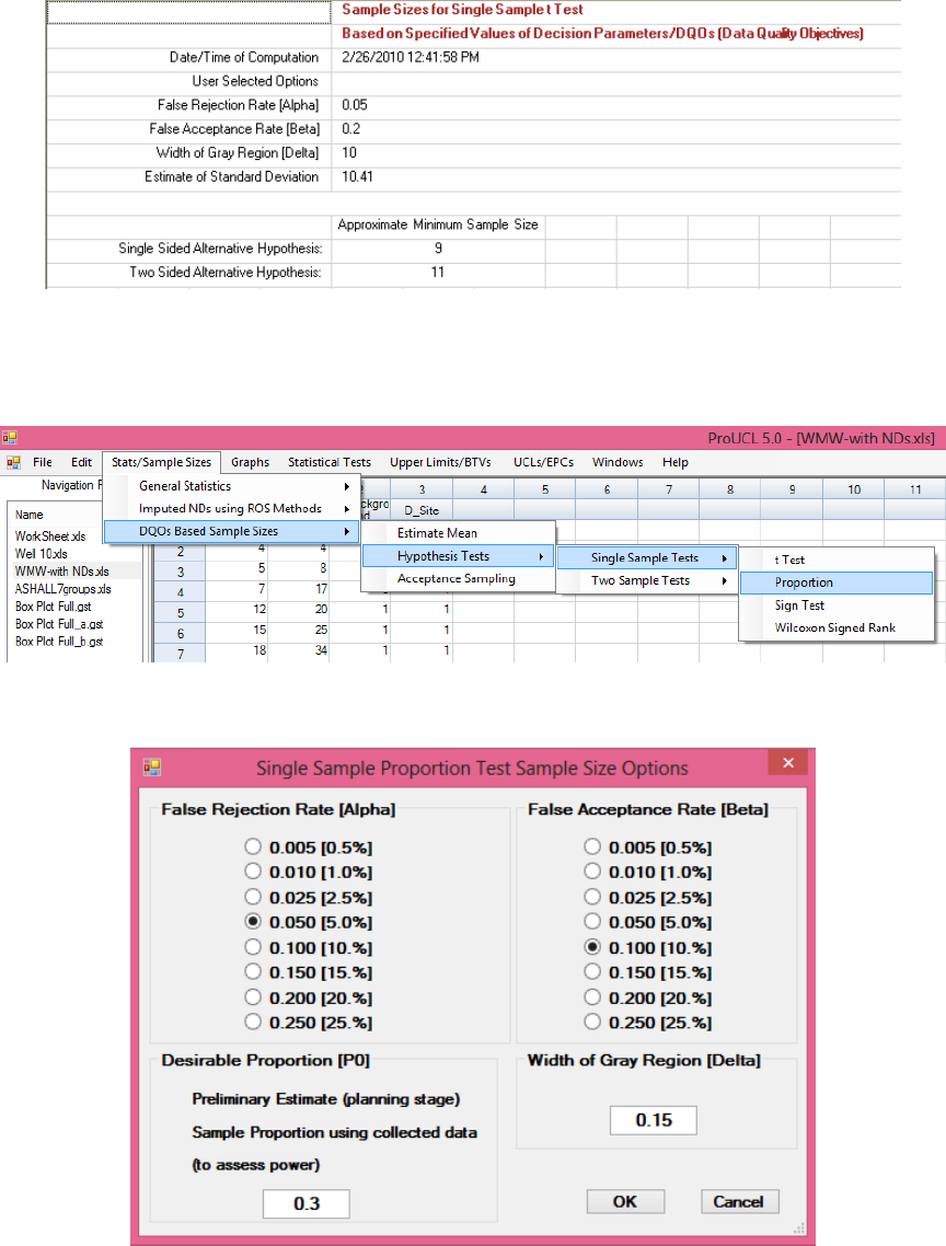
216
Output Screen for Sample Sizes for Single-Sample t-Test (α = 0.05, β = 0.2, sd = 10.41, Δ = 10)
Example from EPA 2006a (page 49)
12.2.2 Sample Size for Single-Sample Proportion Test
1. Click DQOs Based Sample Sizes ► Hypothesis Tests► Single Sample Tests► Proportion
2. The following options window is shown.
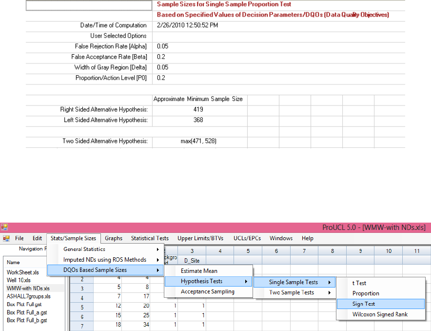
217
Specify the False Rejection Rate (Alpha, α). Default is 0.05.
Specify the False Acceptance Rate (Beta, β). Default is 0.1.
Specify the Desirable Proportion (P0). Default is 0.3.
Specify the Width of the Gray Region (Delta, Δ). Default is 0.15.
Click on OK button to continue or on Cancel button to cancel the options.
Output Screen for Sample Size for Single-Sample Proportion Test (α = 0.05, β = 0.2, P0 = 0.2, Δ =
0.05) Example from EPA 2006a (page 59)
12.2.3 Sample Size for Single-Sample Sign Test
1. Click DQOs Based Sample Sizes ► Hypothesis Tests► Single Sample Tests► Sign Test
2. The following options window is shown.
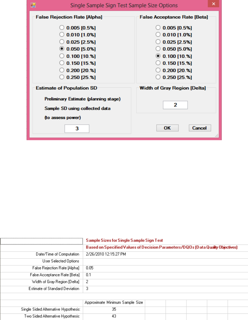
218
Specify the False Rejection Rate (Alpha, α). Default is 0.05.
Specify the False Acceptance Rate (Beta, β). Default is 0.1.
Specify the Estimate of standard deviation. Default is 3
Specify the Width of the Gray Region (Delta, Δ). Default is 2.
Click on OK button to continue or on Cancel button to cancel the options.
Output Screen for Sample Sizes for Single-Sample Sign Test (Default Options)
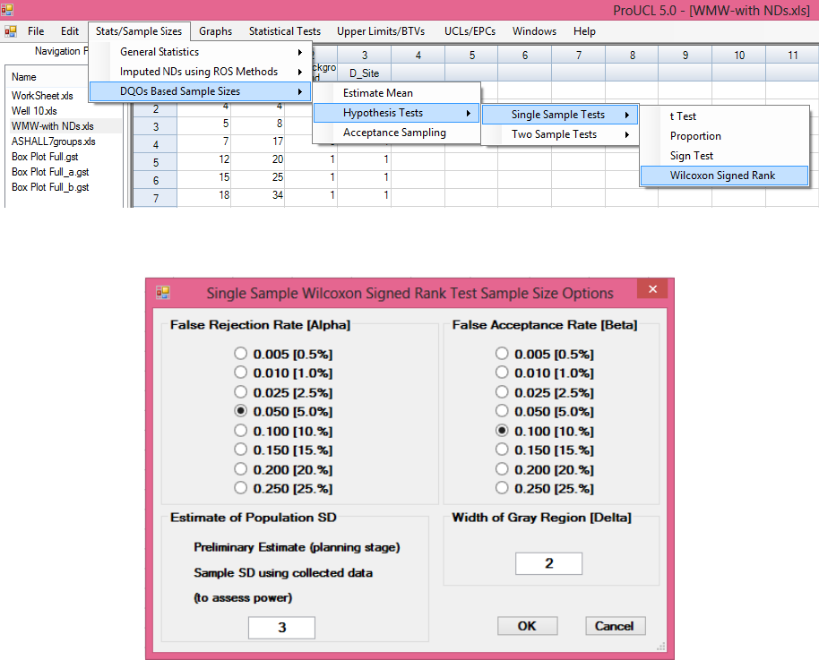
219
12.2.4 Sample Size for Single-Sample Wilcoxon Signed Rank Test
1. Click DQOs Based Sample Sizes ► Hypothesis Tests► Single Sample Tests► Wilcoxon
Signed Rank
2. The following options window is shown.
Specify the False Rejection Rate (Alpha, α). Default is 0.05.
Specify the False Acceptance Rate (Beta, β). Default is 0.1.
Specify the Estimate of standard deviation of WSR Test Statistic. Default is 3
Specify the Width of the Gray Region (Delta, Δ). Default is 2.
Click on OK button to continue or on Cancel button to cancel the options.
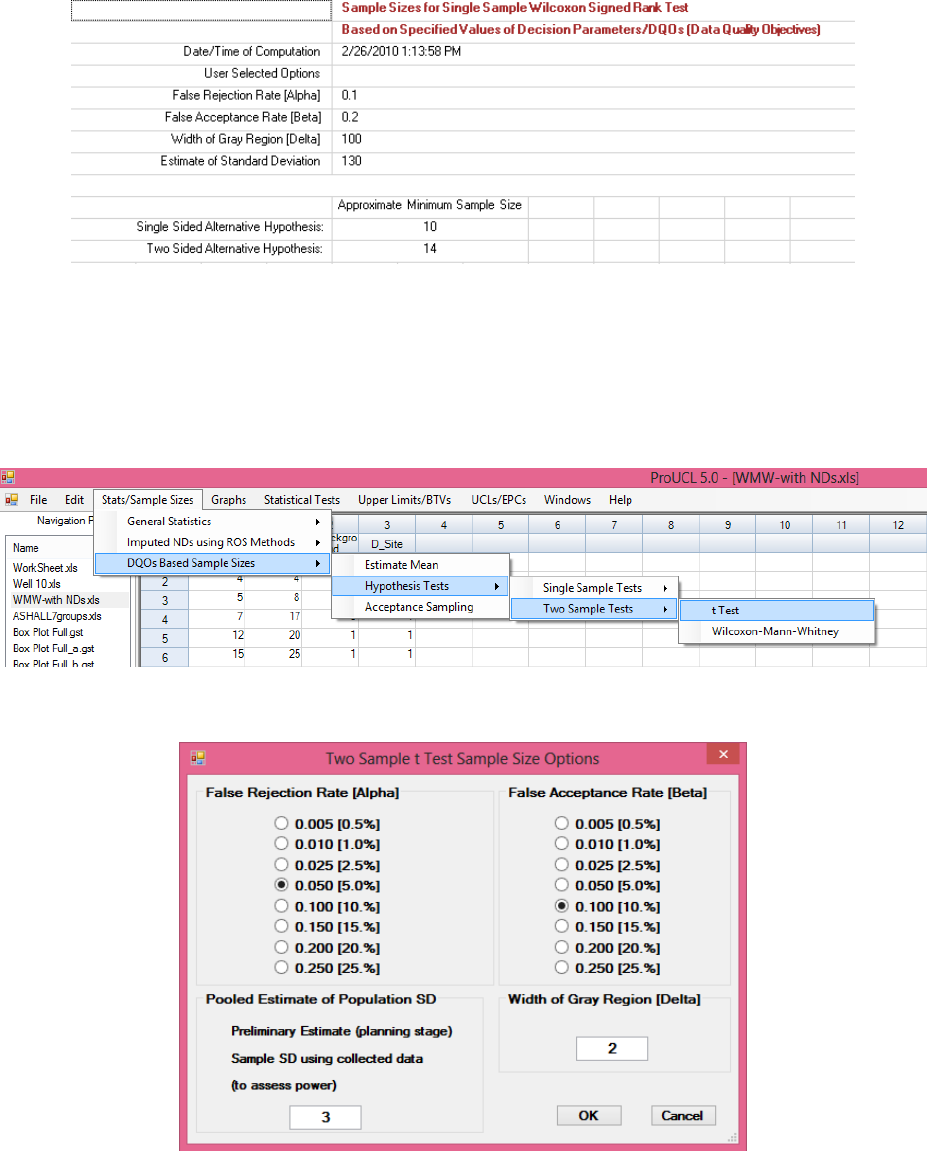
220
Output Screen for Sample Sizes for Single-Sample WSR Test (α = 0.1, β = 0.2, sd = 130, Δ = 100)
Example from EPA 2006a (page 65)
12.3 Sample Sizes for Two-Sample Hypothesis Tests
12.3.1 Sample Size for Two-Sample t-Test
1. Click DQOs Based Sample Sizes ► Hypothesis Tests► Two Sample Tests► t Test
The following options window is shown.
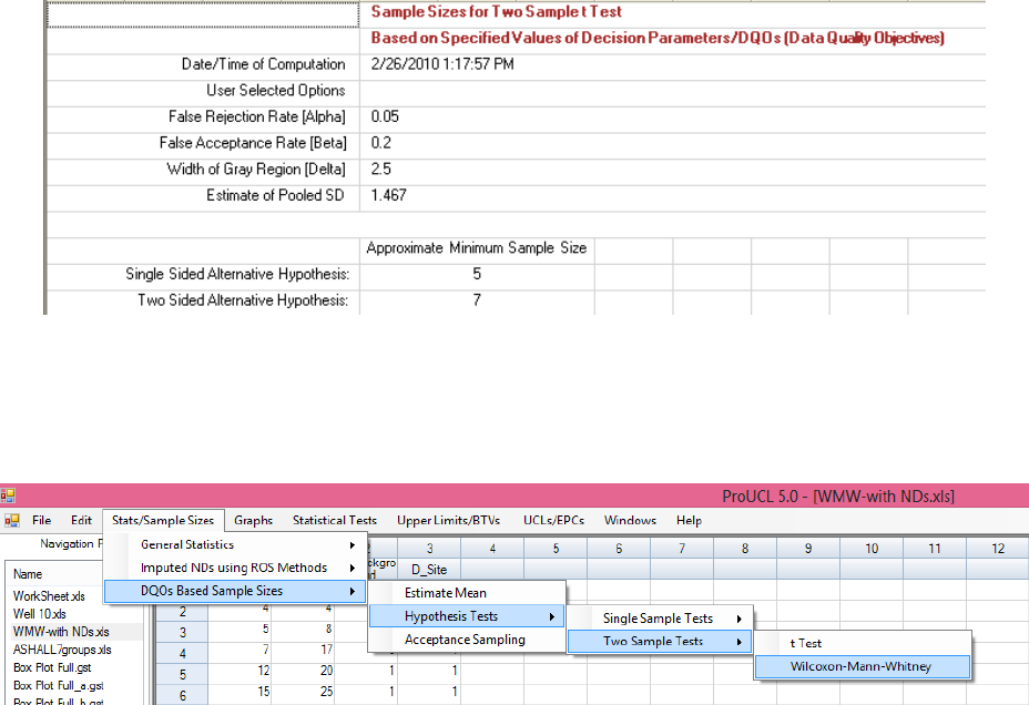
221
Specify the False Rejection Rate (Alpha, α). Default is 0.05.
Specify the False Acceptance Rate (Beta, β). Default is 0.1.
Specify the Estimate of standard deviation. Default is 3
Specify the Width of the Gray Region (Delta, Δ). Default is 2.
Click on OK button to continue or on Cancel button to cancel the options.
Output Screen for Sample Sizes for Two-Sample t-Test (α = 0.05, β = 0.2, s
p
= 1.467, Δ = 2.5)
Example from EPA 2006a (page 68)
12.3.2 Sample Size for Two-Sample Wilcoxon Mann-Whitney Test
1. Click DQOs Based Sample Sizes ► Hypothesis Tests► Two Sample Tests►
Wilcoxon-Mann-Whitney
2. The following options window is shown.
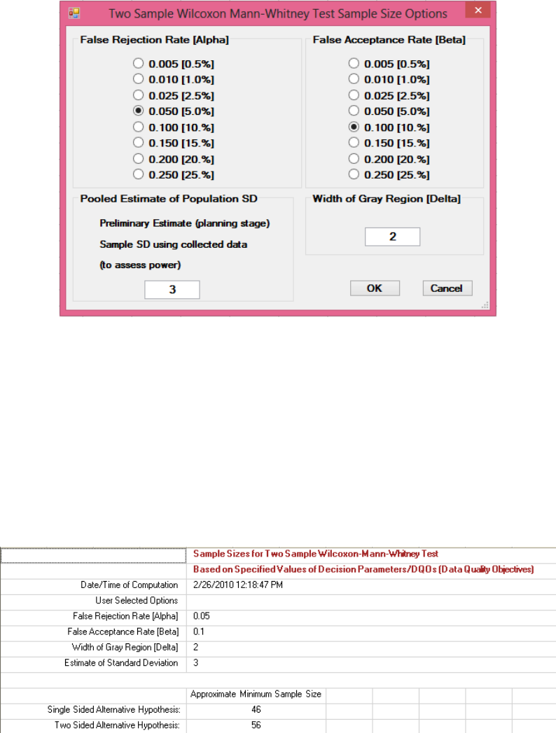
222
Specify the False Rejection Rate (Alpha, α). Default is 0.05.
Specify the False Acceptance Rate (Beta, β). Default is 0.1.
Specify the Estimate of standard deviation of WMW Test Statistic. Default is 3
Specify the Width of the Gray Region (Delta, Δ). Default is 2.
Click on OK button to continue or on Cancel button to cancel the options.
Output Screen for Sample Sizes for Single-Sample WMW Test (Default Options)
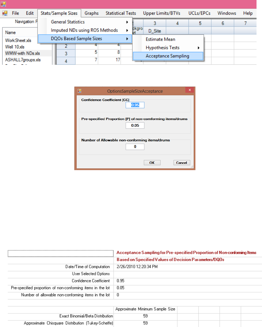
223
12.4 Sample Sizes for Acceptance Sampling
1. Click DQOs Based Sample Sizes ► Acceptance Sampling
2. The following options window is shown.
Specify the Confidence Coefficient. Default is 0.95.
Specify the Proportion [P] of non-conforming items/drums. Default is 0.05.
Specify the Number of Allowable non-conforming items/drums. Default is 0.
Click on OK button to continue or on Cancel button to cancel the options.
Output Screen for Sample Sizes for Acceptance Sampling (Default Options)
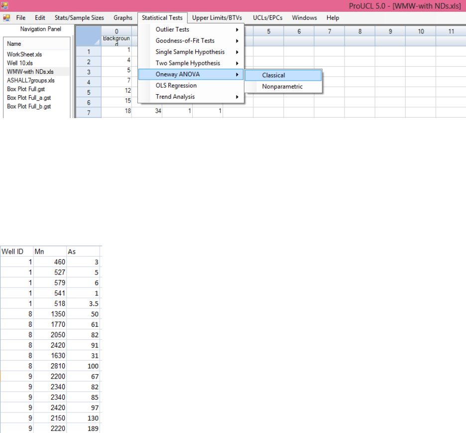
224
Chapter 13
Analysis of Variance
Oneway Analysis of Variance (ANOVA) is a statistical technique that is used to compare the measures of
central tendencies: means or medians of more than two populations/groups. Oneway ANOVA is often
used to perform inter-well comparisons in groundwater monitoring projects. Classical Oneway ANOVA
is a generalization of the two-sample t-test (Hogg and Craig 1995); and nonparametric ANOVA, Kruskal-
Wallis test (Hollander and Wolfe 1999) is a generalization of the two- sample Wilcoxon Mann Whitney
test. Theoretical details of Oneway ANOVA are given in the ProUCL Technical Guide. Oneway
ANOVA is available under the Statistical Tests module of ProUCL 5.0/ProUCL 5.1. It is advised to use
these tests on raw data in the original scale without transforming the data (e.g., using a log-
transformation).
13.1 Classical Oneway ANOVA
1. Click Oneway ANOVA ► Classical
The data file used should follow the format as shown below; the data file should consist of a group
variable defining the various groups (stacked data) to be evaluated using the Oneway ANOVA module.
The Oneway ANOVA module can process multiple variables simultaneously.

225
2. The Select Variables screen will appear.
Select the variables for testing.
Select a Group variable by using the arrow under the Group Column option.
Click OK to continue or Cancel to cancel the test.
Example 13-1a. Consider Fisher’s (1936) 3 species (groups) Iris flower data set. Fisher collected data on
sepal length, sepal width, petal length and petal width for each of the 3 species. Oneway ANOVA results
with conclusions for the variable sepal-width (sp-width) are shown as follows:
Output for a Classical Oneway ANOVA
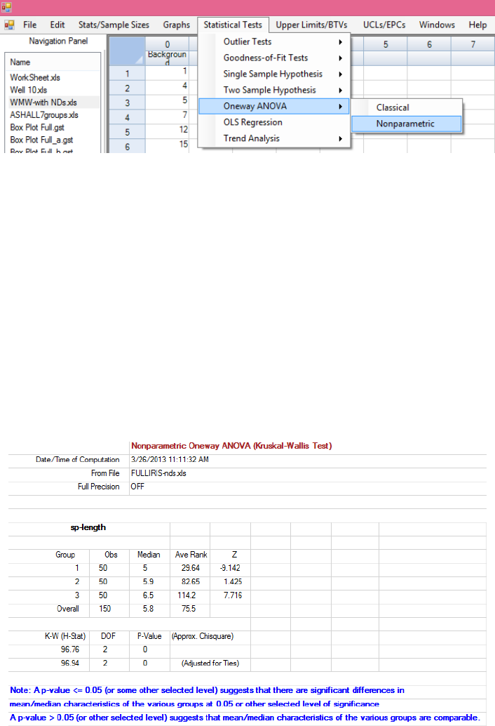
226
13.2 Nonparametric ANOVA
Nonparametric Oneway ANOVA or the Kruskal–Wallis (K-W) test is a generalization of the Mann-
Whitney two-sample test. This is a nonparametric test and can be used when data from the various groups
are not normally distributed.
1. Click Oneway ANOVA ► Nonparametric
Like classical Oneway ANOVA, nonparametric ANOVA also requires that the data file used should
follow the data format as shown above; the data file should consist of a group variable defining the
various groups to be evaluated using the Oneway ANOVA module.
2. The Select Variables screen will appear.
Select the variables for testing.
Select the Group variable.
Click OK to continue or Cancel to cancel the test.
Example 13-1b (continued). Nonparametric Oneway ANOVA results with conclusion for sepal-length
(sp-length) are shown as follows.
Output for a Nonparametric ANOVA
227
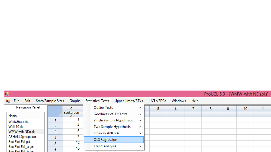
228
Chapter 14
Ordinary Least Squares of Regression and Trend Analysis
The OLS of regression and trend tests are often used to determine trends potentially present in constituent
concentrations at polluted sites, especially in GW monitoring applications. The OLS regression and two
nonparametric trend tests: Mann-Kendall test and Theil-Sen test are available under the Statistical Tests
module of ProUCL 5.0/ProUCL 5.1. The details of these tests can be found in Hollander and Wolfe
(1999) and Draper and Smith (1998). Some time series plots, which are useful in comparing trends in
analyte concentrations of multiple groups (e.g., monitoring wells), are also available in ProUCL.
The two nonparametric trend tests: M-K test and Theil-Sen test are meant to identify trends in time series
data (data collected over a certain period of time such as daily, monthly, quarterly, etc.) with distinct
values of the time variable (time of sampling events). If multiple observations are collected/reported at a
sampling event (time), one or more pairwise slopes used in the computation of the Theil-Sen test may not
be computed (become infinite). Therefore, it is suggested that the Theil-Sen test only be used on data sets
with one measurement collected at each sampling event. If multiple measurements are collected at a
sampling event, the user may want to use the average (or median, mode, minimum or maximum) of those
measurements resulting in a time series with one measurement per sampling time event. Theil-Sen test in
ProUCL has an option which can be used to average multiple observations reported for the various
sampling events. The use of this option also computes M-K test statistic and OLS statistics based upon
averages of multiple observations collected at the various sampling events.
New in ProUCL 5.1: In addition to slope and intercept of the nonparametric Theil-Sen (T-S) trend line,
ProUCL 5.1 computes residuals based upon the T-S trend line.
The trend tests in ProUCL software also assume that the user has entered data in chronological order. If
the data are not entered properly in chronological order, the graphical trend displays may be meaningless.
Trend Analysis and OLS Regression modules handle missing values in both response variable (e.g.,
analyte concentrations) as well as the sampling event variable (called independent variable in OLS).
14.1 Simple Linear Regression
1. Click Statistical Tests► OLS Regression.
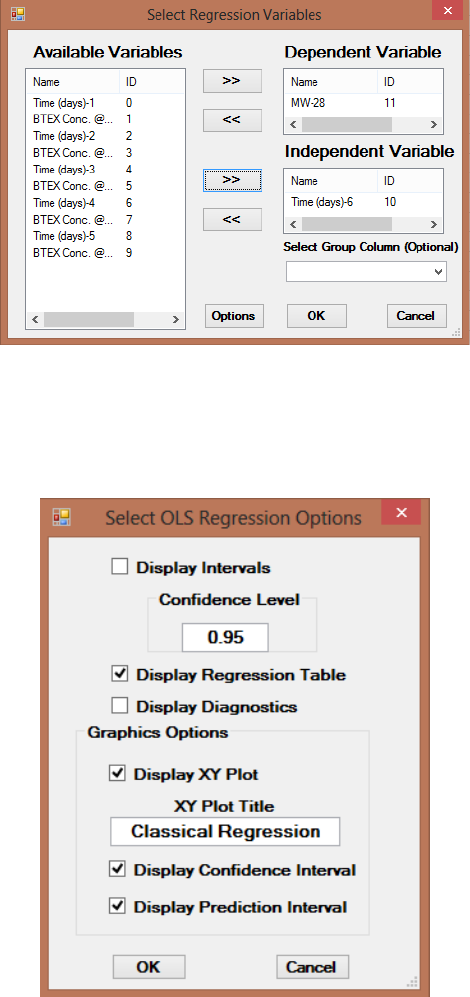
229
2. The Select Regression Variables screen will appear.
Select the Dependent Variable and the Independent Variable for the regression analysis.
Select a group variable (if any) by using the arrow below the Select Group Column
(Optional). The analysis will be performed separately for each group.
When the Options button is clicked, the following options window will appear.
o Select Display Intervals for the confidence limits and the prediction limits of each
observation to be displayed at the specified Confidence Coefficient. The interval
estimates will be displayed in the output sheet.
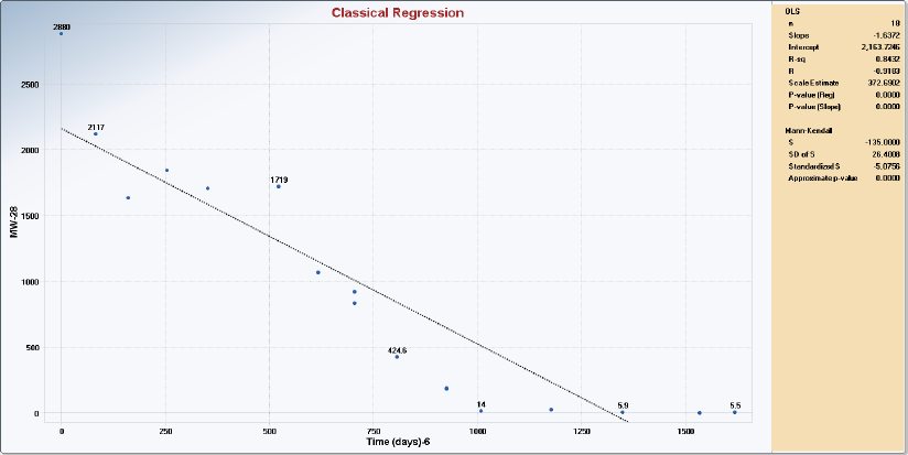
230
o Select Display Regression Table to display Y-hat, residuals and the standardized
residuals in the output sheet.
o Select “XY Plot” to generate a scatter plot display showing the regression line.
o Select Confidence Interval and Prediction Interval to display the confidence and
the prediction bands around the regression line.
o Click on OK button to continue or on Cancel button to cancel the option.
Click OK to continue or Cancel to cancel the OLS Regression.
o The use of the above options will display the following graph on your computer
screen which can be copied using the Copy Chart (To Clipboard) in a Microsoft
documents (e.g., word document) using the File ►Paste combination.
o The above options will also generate an Excel-Type output sheet. A partial output
sheet is shown below following the OLS Regression Graph.
Example 14-1a. Consider analyte concentrations, X collected from a groundwater (GW) monitoring well,
MW-28 over a certain period of time. The objective is to determine if there is any trend in GW
concentrations, X of the MW-28. The OLS regression line with inference about slope and intercept are
shown in the following figure. The slope and its associated p-value suggest that there is a significant
downward trend in GW concentrations of MW-28.
OLS Regression Graph without Regression and Prediction Intervals
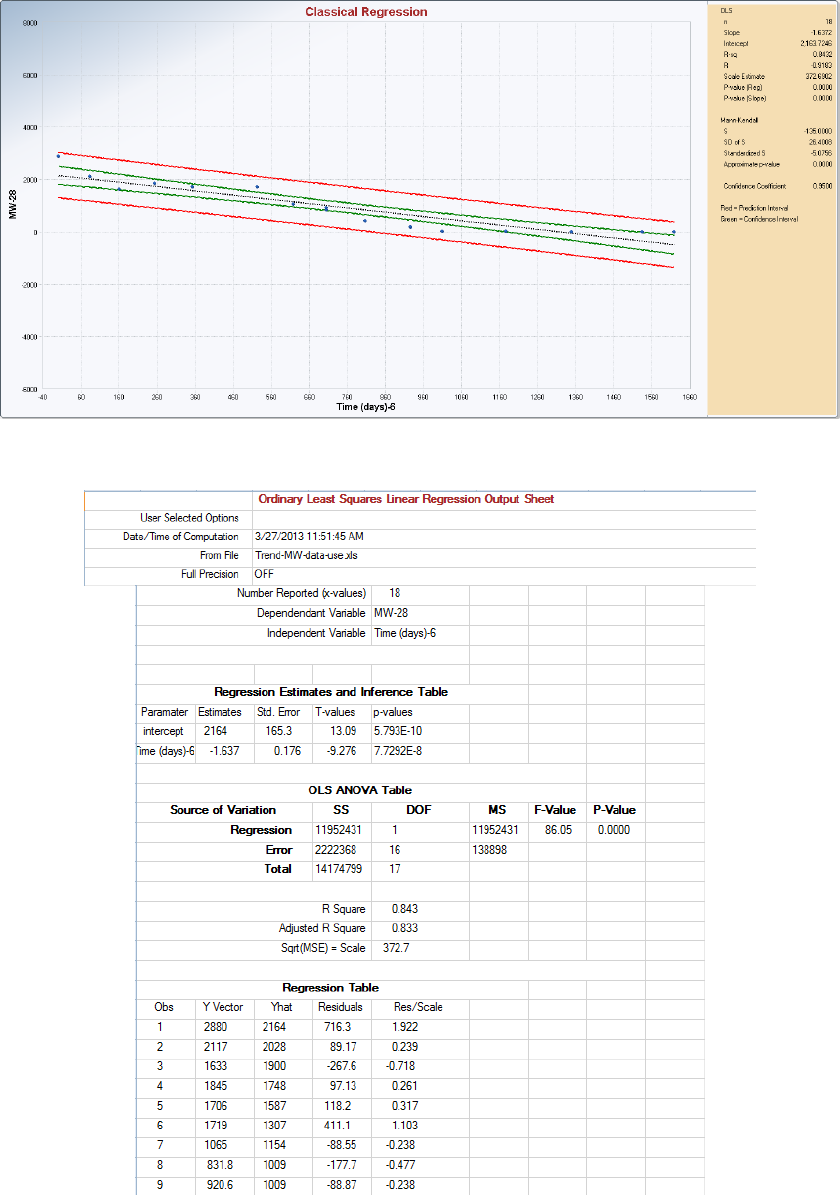
231
OLS Regression Graph with Regression and Prediction Intervals
Partial Output of OLS Regression Analysis
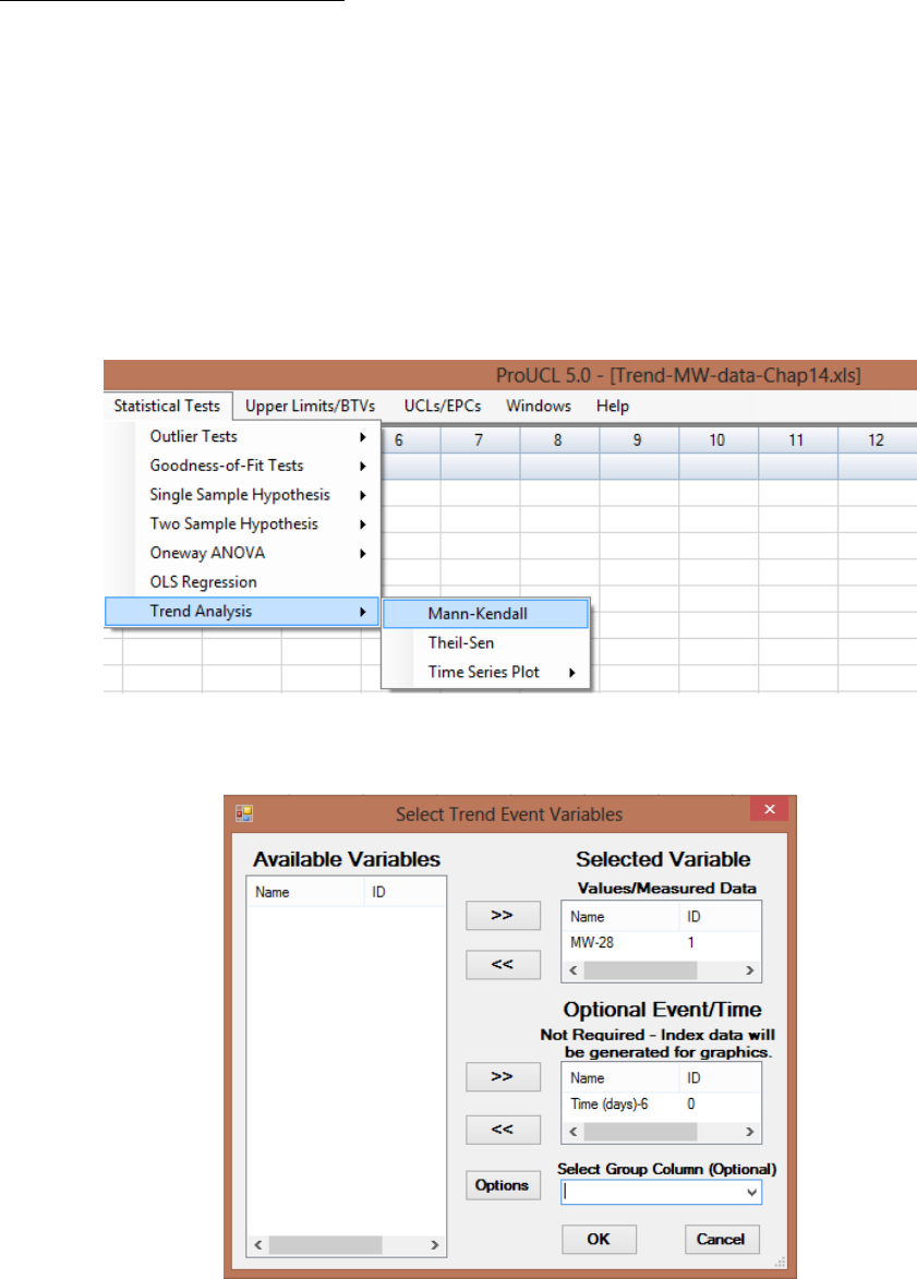
232
Verifying Normality of Residuals: As shown in the above partial output, ProUCL displays residuals
including standardized residuals on the OLS output sheet. Those residuals can be imported (copying and
pasting) in an excel file to assess the normality of those OLS residuals. The parametric trend evaluations
based upon the OLS slope (significant slope, confidence interval and prediction interval) are valid
provided the OLS residuals are normally distributed. Therefore, it is suggested that the user assesses the
normality of OLS residuals before drawing trend conclusions using a parametric test based upon the OLS
slope estimate. When the assumptions are not met, one can use graphical displays and nonparametric
trend tests (e.g., T-S test) to determine potential trends present in a time series data set.
14.2 Mann-Kendall Test
1. Click Statistical Tests ►Trend Analysis ► Mann-Kendall.
2. The Select Trend Event Variables screen will appear.
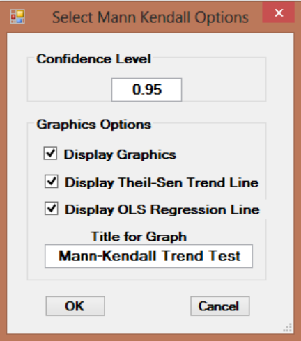
233
Select the Event/Time variable. This variable is optional to perform the Mann-Kendall
(M-K) Test; however, for graphical display it is suggested to provide a valid Event/Time
variable (numerical values only). If the user wants to generate a graphical display without
providing an Event/Time variable, ProUCL generates an index variable to represent
sampling events.
Select the Values/Measured Data variable to perform the trend test.
Select a group variable (if any) by using the arrow below the Select Group Column
(Optional). When a group variable is chosen, the analysis is performed separately for
each group represented by the group variable.
When the Options button is clicked, the following window will be shown.
o Specify the Confidence Level; a number in the interval (0.5, 1), 0.5 inclusive. The
default choice is 0.95.
o Select the trend lines to be displayed: OLS Regression Line and/or Theil-Sen
Trend Line. If only Display Graphics is chosen, a time series plot will be generated.
o Click on OK button to continue or on Cancel button to cancel the option.
Click OK to continue or Cancel to cancel the Mann-Kendall test.
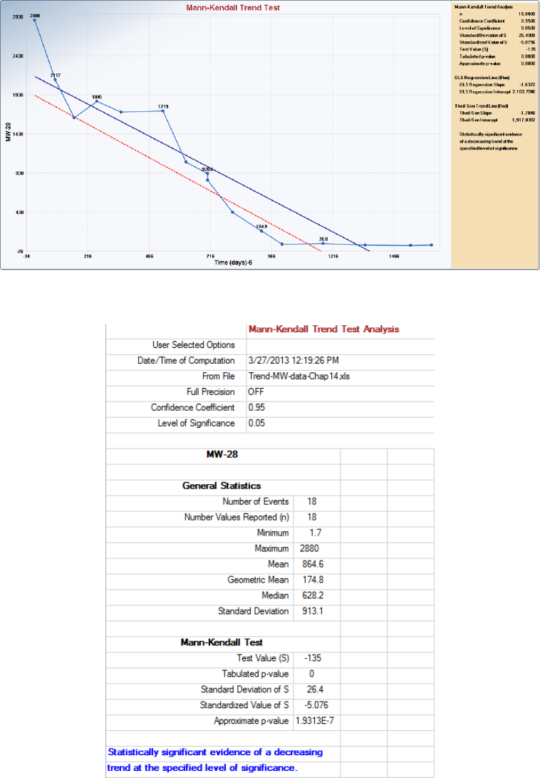
234
14- 1b (Continued). The M-K test results are shown in the following figure and in the following M-K
test output sheet. Based upon the M-K test, it is concluded that there is a statistically significant
downward trend in GW concentrations of the MW-28.
Mann Kendall Test Trend Graph displaying all Selected Options
Mann-Kendall Trend Test Output Sheet
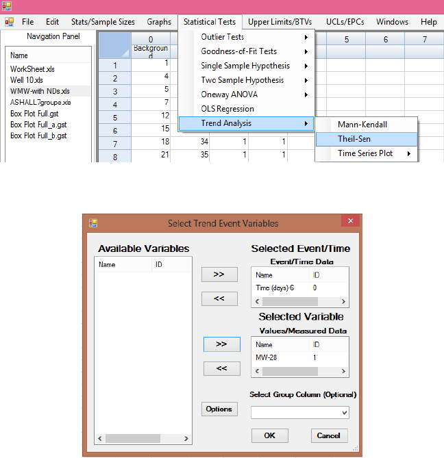
235
14.3 Theil – Sen Test
To perform the Theil-Sen test, the user is required to provide numerical values for a sampling event
variable (numerical values only) as well as values of a characteristic (e.g., analyte concentrations) of
interest observed at those sampling events.
1. Click Statistical Tests ►Trend Analysis ► Theil-Sen.
2. The Select Variables screen will appear.
Select an Event/Time Data variable.
Select the Values/Measured Data variable to perform the test.
Select a group variable (if any) by using the arrow below the Select Group Column
(Optional). When a group variable is chosen, the analysis is performed separately for
each group represented by the group variable.
When the Options button is clicked, the following window will be shown.
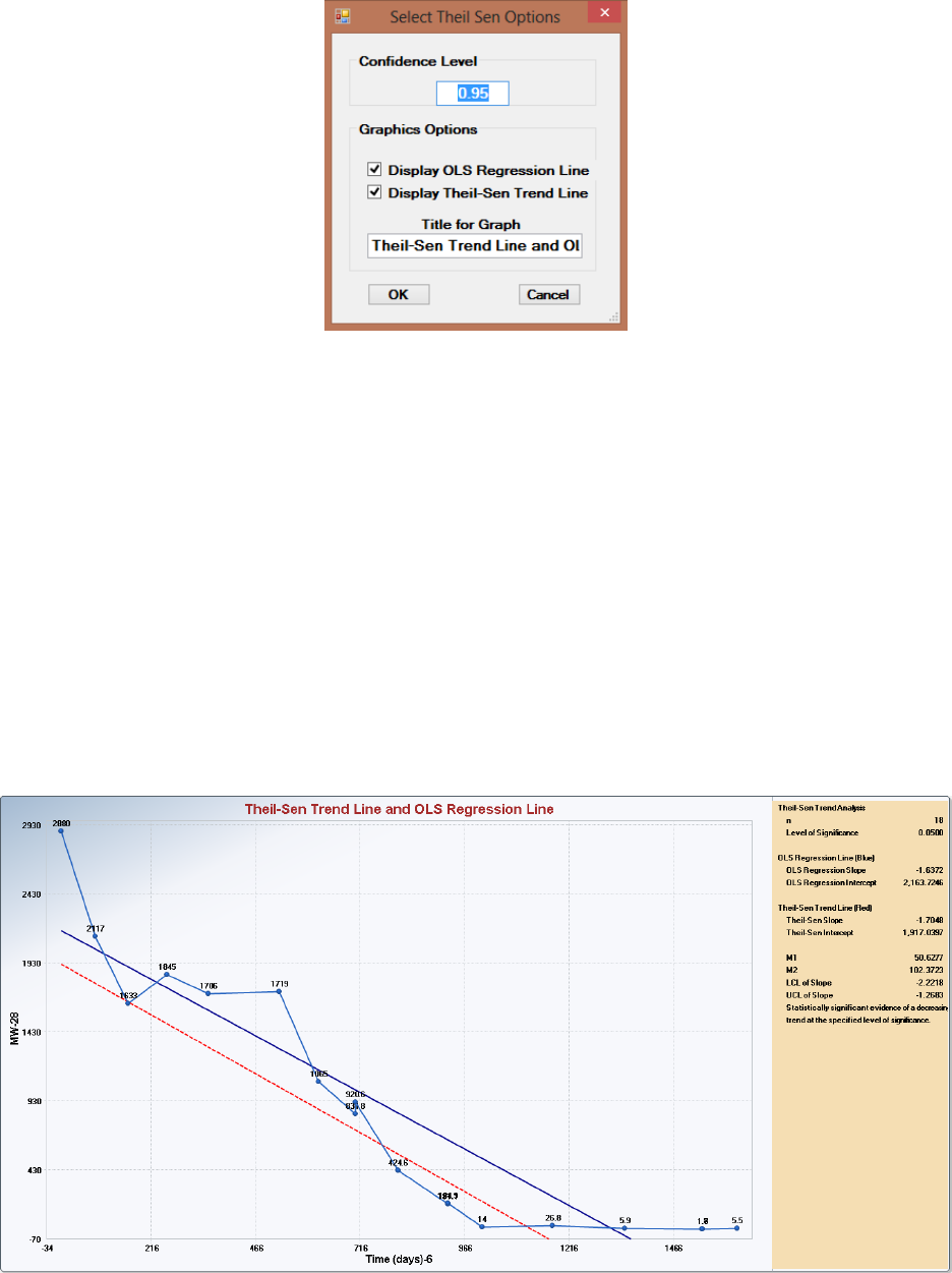
236
o Specify the Confidence Level; a number in the interval (0.5, 1), 0.5 inclusive. The
default choice is 0.95.
o Select the trend lines to be displayed: OLS Regression Line and/or Theil-Sen
Trend Line.
o Click on OK button to continue or on Cancel button to cancel the option.
Click OK to continue or Cancel to cancel the Theil-Sen Test.
14-1c (continued). The Theil-Sen test results are shown in the following figure and in the following
Theil-Sen test Output Sheet. It is concluded that there is a statistically significant downward trend in GW
concentrations of MW-28. Theil-Sen test results and residuals are summarized in tables following the
trend graph shown below.
Theil-Sen Test Trend Graph displaying all Selected Options
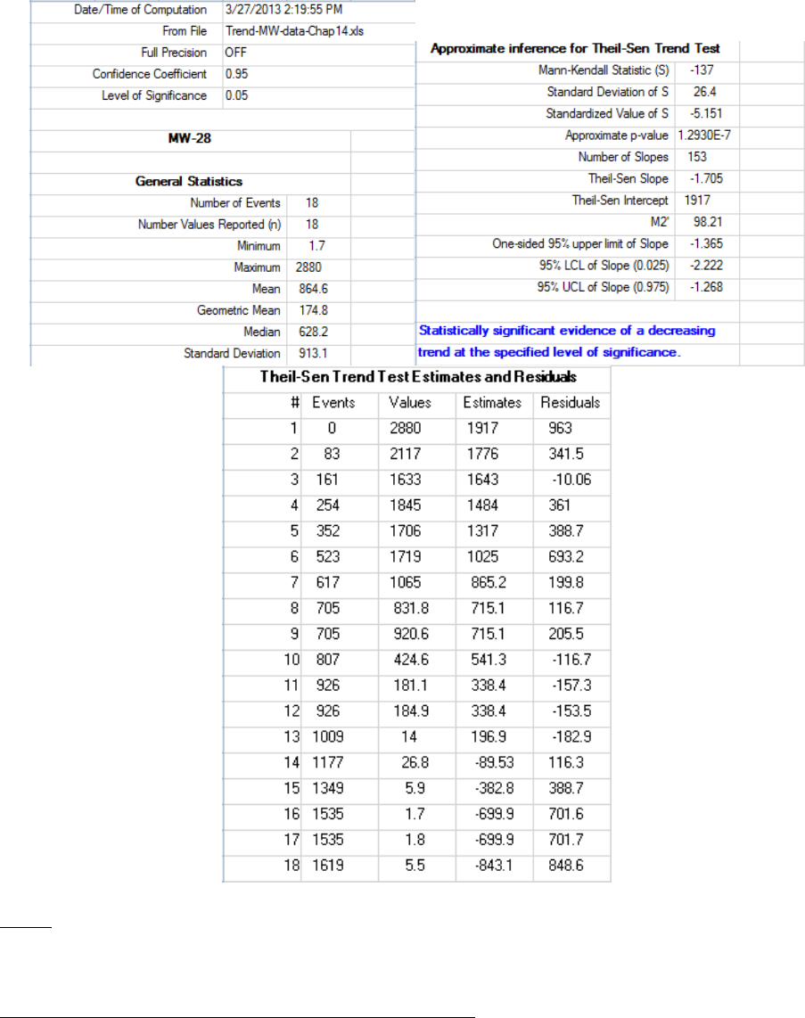
237
Theil-Sen Trend Test Output Sheet
Notes: As with other statistical test statistics, trend test statistics: M-K test statistic, OLS regression and
Theil-Sen slopes may lead to different trend conclusions. In such instances it is suggested that the user
supplements statistical conclusions with graphical displays.
Averaging of Multiple Measurements at Sampling Events: In practice, when multiple observations are
collected/reported at one or more sampling events (times), one or more pairwise slopes may become
infinite, resulting in a failure to compute the Theil-Sen test statistic. In such cases, the user may want to
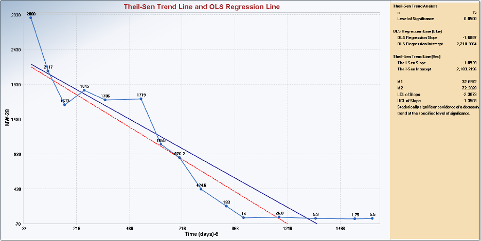
238
pre-process the data before using the Theil-Sen test. Specifically, to assure that only one measurement is
available at each sampling event, the user pre-processes the time series data by computing average,
median, mode, minimum, or maximum of the multiple observations collected at those sampling events.
The Theil-Sen test in ProUCL 5.0/ProUCL 5.1 provides the option of averaging multiple measurements
collected at the various sampling events. This option also computes M-K test and OLS regression
statistics using the averages of multiple measurements collected at the various sampling event. The OLS
regression and M-K test can be performed on data sets with multiple measurements taken at the various
sampling time events. However, often it is desirable to use the averages (or median) of measurements
taken at the various sampling events to determine potential trends present in a time-series data set.
14-1c (continued). The data set used in Example 14-1c has some sampling events where multiple
observations were taken. Theil-Sen test results based upon averages of multiple observations is shown as
follows. The data set is included in the ProUCL Data directory which comes with ProUCL 5.1.
Theil-Sen Test Trend Graph displaying all Selected Options
Multiple Observations Taken at Some Sampling Events Have Been Averaged
14.4 Time Series Plots
This option of the Trend Analysis module can be used to determine and compare trends in multiple
groups over the same period of time.
This option is specifically useful when the user wants to compare the concentrations of multiple groups
(wells) and the exact sampling event dates are not be available (data only option). The user may just want
to graphically compare the time-series data collected from multiple groups/wells during several quarters
(every year, every 5 year, etc.). When the user wants to use this module using the data/event option,
each group (e.g., well) defined by a group variable must have the same number of observations and
should share the same sampling event values. That is the number of sampling events and values (e.g.,
quarter ID, year ID, etc.) for each group (well) must be the same for this option to work. However, the
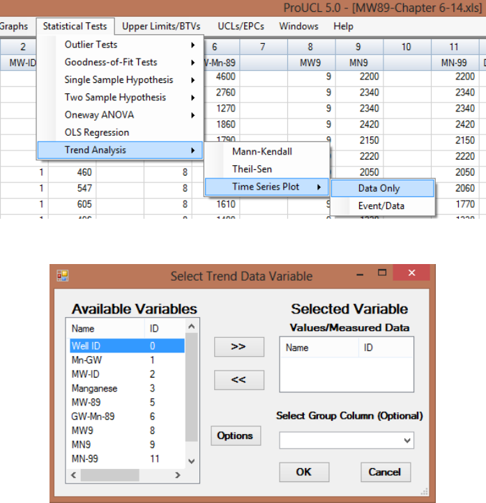
239
exact sampling dates (not needed to use this option) in the various quarters (years) do not have to be the
same as long as the values of the sampling quarters/years (1,3,5,6,7,9,..) used in generating time-series
plots for the various groups (wells) match. Using the geological and hydrological information, this kind of
comparison may help the project team in identifying non-compliance wells (e.g., with upward trends in
constituent concentrations) and associated reasons.
1. Click Statistical Tests ►Trend Analysis ► Time Series Plots
2. When the Data Only option is clicked, the following window is shown:
This option is used on the measured data only. The user selects a variable with measured values
which are used in generating a time series plot. The time series plot option is specifically useful
when data come from multiple groups (monitoring wells during the same period of time).
Select a group variable (is any) by using the arrow shown below the Group Column (Optional).

240
When the Options button is clicked, the following window will be shown.
The user can opt to display graphs for each group individually or for all groups together on the
same graph by selecting the Group Graphs option. The user can also display the OLS line and/or
the Theil-Sen line for all groups displayed on the same graph. The user may pick an initial
starting value and an increment value to display the measured data. All statistics will be computed
using the data displayed on the graphs (e.g., selected Event values).
o Input a starting value for the index of the plot using the Set Initial Start Value.
o Input the increment steps for the index of the plot using the Set Index/Event Increments.
o Specify the lines (Regression and/or Theil-Sen) to be displayed on the time series plot.
o Select Plot Graphs Together option for comparing the time series trends for more than one
group on the same graph.
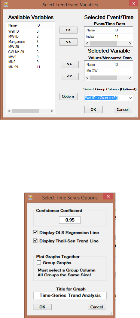
241
o If this option is not selected but a Group Variable is selected, different graphs will be plotted
for each group.
o Click on OK button to continue or on Cancel button to cancel the Time Series Plot.
3. When the Event/Data option is clicked, the following window is shown:
Select a group variable (is any) by using the arrow shown below the Group Column (Optional).
This option uses both the Measured Data and the Event/Time Data. The user selects two
variables; one representing the Event/Time variable and the other representing the Measured Data
values which will be used in generating a time series plot.
When the Options button is clicked, the following window will be shown.
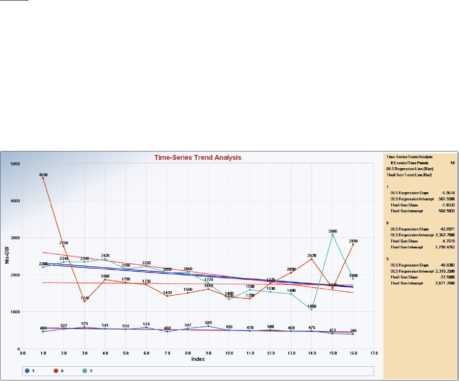
242
The user can select to display graphs individually or together for all groups on the same graph by
selecting the Plot Graphs Together option. The user can also display the OLS line and/or the
Theil-Sen line for all groups displayed on the same graph.
o Specify the lines (Regression and/or Theil-Sen) to be displayed on the time series plot.
o Select Plot Graphs Together option for comparing time series trends for more than one
group on the same graph.
o If this option is not selected but a Group Variable is selected, different graphs will be plotted
for each group.
o Click on OK button to continue or on Cancel button to cancel the options.
Click OK to continue or Cancel to cancel the Time Series Plot.
Notes: To use this option, each group (e.g., well) defined by a group variable must have the same number
of observations and should share the same sampling event values (if available). That is the sampling
events (e.g., quarter ID, year ID, etc.) for each group (well) must be the same for this option to work.
Specifically, the exact sampling dates within the various quarters (years) do not have to be the same as
long as the sampling quarters (years) for the various wells match.
Example 14-2. The following graph has three (3) time series plots comparing manganese concentrations
of the three GW monitoring wells (1 upgradient well [MW1] and 2 downgradient wells [MW8 and
MW9]) over the period of 4 years (data collected quarterly). Some trend statistics are displayed in the
side panel.
Output for a Time Series Plot – Event/Data Option by a Group Variable (1, 8, and 9)
243

244
Chapter 15
Background Incremental Sample Simulator (BISS)
Simulating BISS Data from a Large Discrete Background Data
The Background Incremental Sample Simulator (BISS) module was incorporated in ProUCL5.0 at the
request of the Office of Superfund Remediation and Technology Innovation (OSRTI). However, this
module is currently under further investigation and research, and therefore it is not available for general
public use. This module has been retained in ProUCL 5.1. This module may be released in a future
version of the ProUCL software, along with strict conditions and guidance for how it is applied. The main
text for this chapter is not included in this document for release to general public. Only a brief placeholder
write-up is provided here.
The following scenario describes the Site or project conditions under which the BISS module could be
useful: Suppose there is a long history of soil sample collection at a Site. In addition to having a large
amount of Site data, a robust background data set (at least 30 samples from verified background
locations) has also been collected. Comparison of background data to on-Site data has been, and will
continue to be, an important part of this project’s decision-making strategy. All historical data is from
discrete samples, including the background data. There is now a desire to switch to incremental sampling
for the Site. However, guidance for incremental sampling makes it clear that it is inappropriate to
compare discrete sample results to incremental sample results. That includes comparing a Site’s
incremental results directly to discrete background results.
One option is to recollect all background data in the form of incremental samples from background DUs
that are designed to match Site DUs in geology, area, depth, target soil particle size, number of
increments, increment sample support, etc. If project decision-making uses a BTV strategy to compare
Site DU results one at a time against background, then an appropriate number (the default is no less than
10) of background DU incremental samples would need to be collected to determine the BTV for the
population of background DUs. However, if the existing discrete background data show background
concentrations to be low (in comparison to Site concentrations) and fairly consistent (relative standard
deviation, RSD <1), there is a second option described as follows.
When a robust discrete background data set that meets the above conditions already exists, the following
is an alternative to automatically recollecting ALL background data as incremental samples.
Step 1. Identify 3 background DUs and collect at least 1 incremental sample from each for a minimum of
3 background incremental samples.
Step 2. Enter the discrete background data set (n 30) and the 3 background incremental samples into
the BISS module (the BISS module will not run unless both data sets are entered).
The BISS module will generate a specified (default is 7) simulated incremental samples from the
discrete data set.
The module will then run a t-test to compare the simulated background incremental data set (e.g.,
with n = 7) to the actual background incremental data set (n 3).

245
o If the t-test finds no difference between the 2 data sets, the BISS module will combine
the 2 data sets and determine the statistical distribution, mean, standard deviation,
potential UCLs and potential BTVs for the combined data set. Only this information will
be supplied to the general user. The individual values of the simulated incremental
samples will not be provided.
o If the t-test finds a difference between the actual and simulated data sets, the BISS
module will not combine the data sets nor provide a BTV.
o In both cases, the BISS module will report summary statistics for the actual and
simulated data sets.
Step 3. If the BISS module reported out statistical analyses from the combined data set, select the BTV to
use with Site DU incremental sample results. Document the procedure used to generate the BTV in
project reports. If the BISS module reported that the simulated and actual data sets were different, the
historical discrete data set cannot be used to simulate incremental results. Additional background DU
incremental samples will need to be collected to obtain a background DU incremental data set with the
number of results appropriate for the intended use of the background data set.
The objective of the BISS module is to take advantage of the information provided by the existing
background discrete samples. The availability of a large discrete data set collected from the background
areas with geological formations and conditions comparable to the Site DU(s) of interest is a requirement
for successful application of this module. There are fundamental differences between incremental and
discrete samples. For example, the sample supports of discrete and incremental samples are very
different. Sample support has a profound effect on sample results so samples with different sample
supports should not be compared directly, or compared with great caution.
Since incremental sampling is a relatively new approach, the performance of the BISS module requires
further investigation. If you would like to try this strategy for your project, or if you have questions,
contact Deana Crumbling, crumbling[email protected].
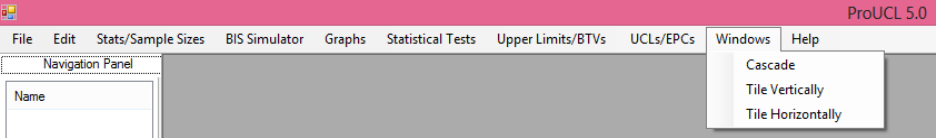
246
Chapter 16
Windows
The Windows Menu performs typical Windows program options.
Click on the Window menu to reveal the drop-down options shown above.
The following Window drop-down menu options are available:
Cascade option: arranges windows in a cascade format. This is similar to a typical
Windows program option.
Tile option: resizes each window vertically or horizontally and then displays all open
windows. This is similar to a typical Windows program option.
The drop-down options list also includes a list of all open windows with a check mark in
front of the active window. Click on any of the windows listed to make that window
active. This is especially useful if you have many windows (e.g., >40) open; the
navigation panel only holds the first 40 windows.
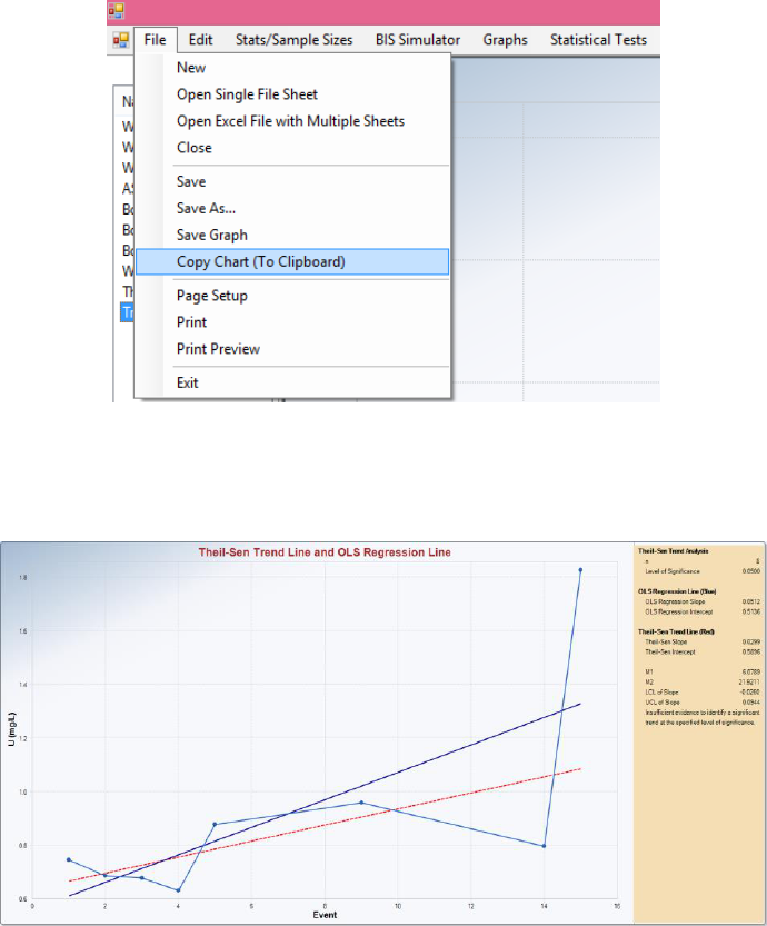
247
Chapter 17
Handling the Output Screens and Graphs
17.1 Copying and Saving Graphs
Graphs can be copied into Word, Excel, or PowerPoint files in two ways.
1. Click the Copy Chart (To Clipboard) shown below; a graph must be present to be copied to the
clipboard.
File ► Copy Chart (To Clipboard)
Once the user has clicked Copy Chart (To Clipboard), the graph is ready to be imported
(pasted) into most Microsoft office applications (e.g., Word, Excel, and PowerPoint) by clicking
the Edit ► Paste option in those Microsoft applications as shown below.
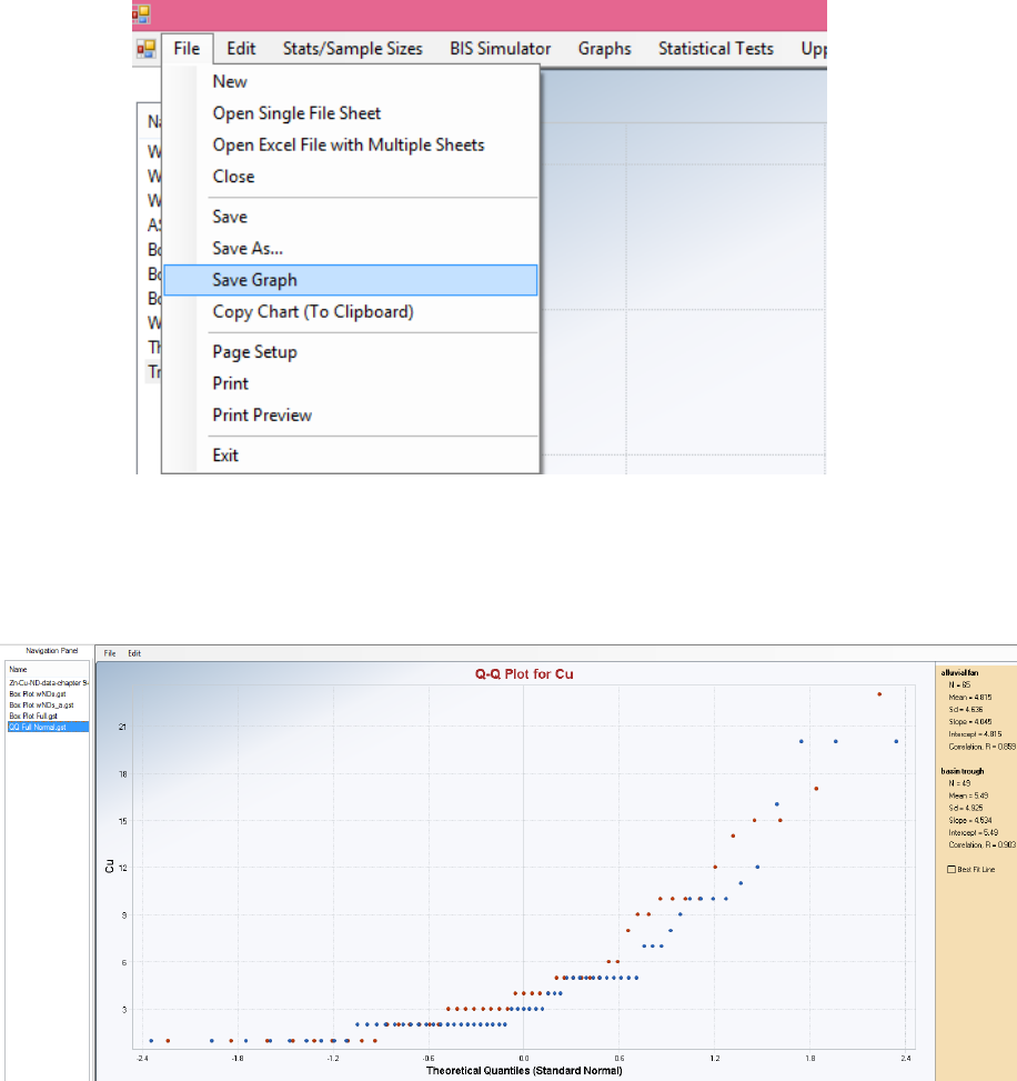
248
2. Graphs can be saved using the Save Graph Option in the Navigation Panel as a Bitmap file
with .bmp extension. The user can import the saved bitmap file into a desired document such as a
word document or a PowerPoint presentation by using the Copy and Paste options available in
the selected Microsoft application.
File ► Save Graph
17.2 Printing Graphs
1. Click the graph you want to print in the Navigation Panel.
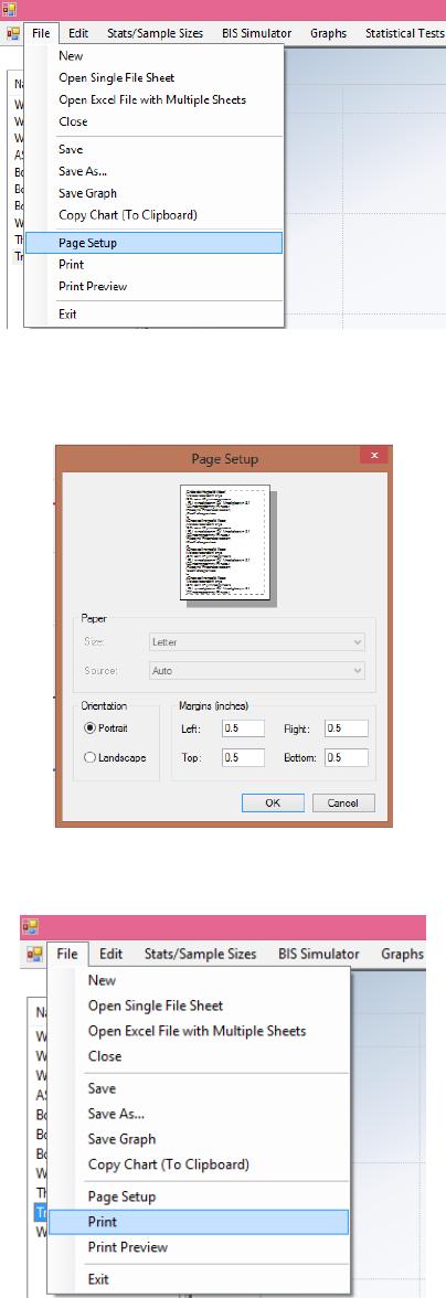
249
2. Click File ► Page Setup.
3. Check the button next to Portrait or Landscape (shown below), and click OK. In some cases,
with larger headings and captions, it may be desirable to use the Landscape printing option.
4. Click File ► Print to print the graph, and File ► Print Preview to preview (optional) the graph
before printing.
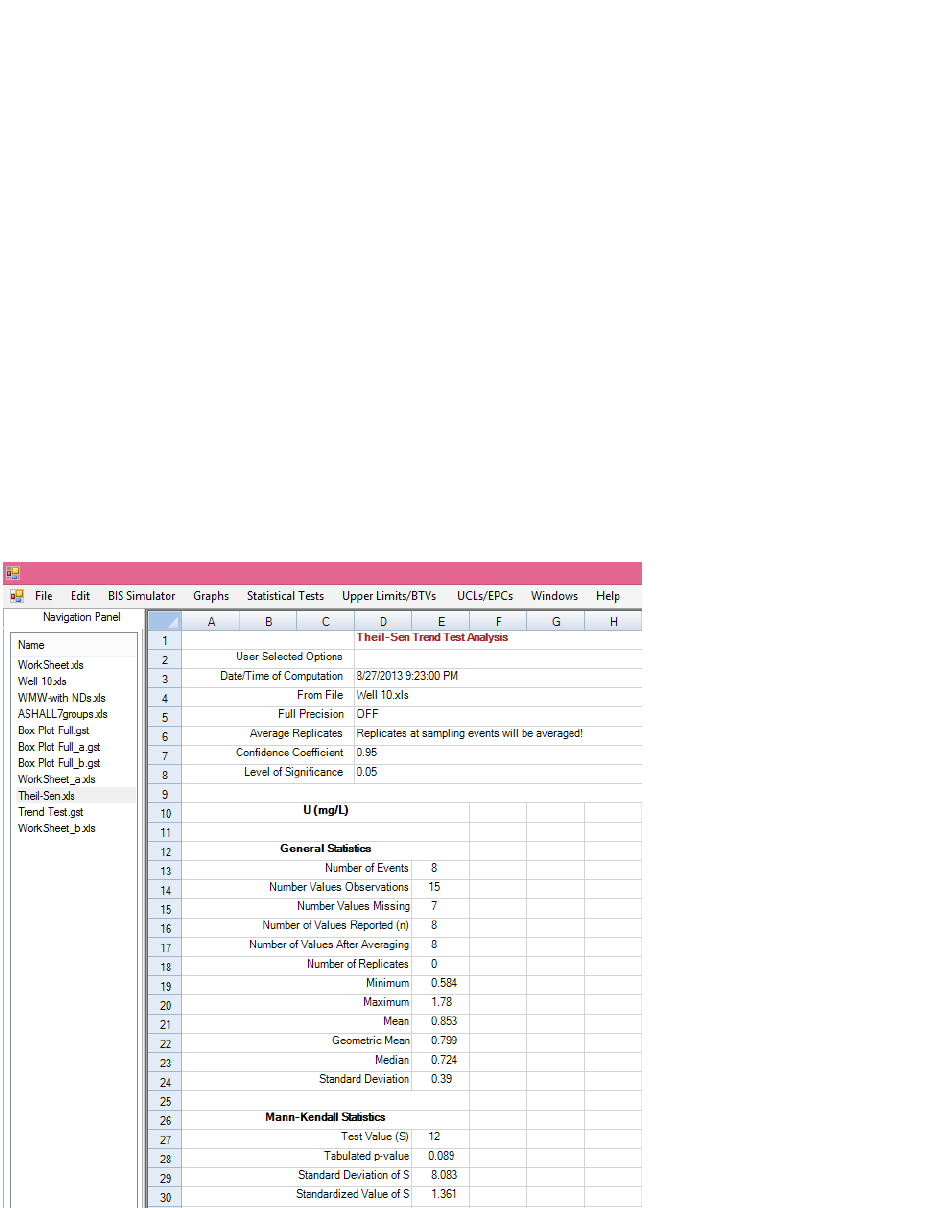
250
17.3 Making Changes in Graphs using Tools and Properties
ProUCL uses a couple of development tools such as FarPoint spread (for Excel type input and output
operations) and ChartFx (for graphical displays). ProUCL generates box plots using the built-in box plot
feature in ChartFx. The programmer has no control over computing various statistics (e.g., Q1, Q2, Q3,
IQR) using ChartFx. So box plots generated by ProUCL can differ slightly from box plots generated by
other programs (e.g., Excel). Box plots generated using ChartFx round values to the nearest integer. For
increased precision of graphical displays (all graphical displays generated by ProUCL), the user can use
the process described as follows.
Position your mouse cursor on the graph and right-click, a popup menu will appear. Position the mouse
on Properties and right-click; a windows form labeled Properties will appear. There are three choices at
the top; General, Series and Y-Axis. Position the mouse cursor over the Y-Axis choice and left-click.
You can change the number of decimals to increase the precision, change the step to increase or decrease
the number Y-Axis values displayed and/or change the direction of the label. To show values on the plot
itself, position your mouse cursor on the graph and right-click; a popup menu will appear. Position the
mouse on Point Labels and right-click. There are other options available in this popup menu including
changing font sizes.
17.4 Printing Non-graphical Outputs
1. Click/Highlight the output you want to save or print in the Navigation Panel.
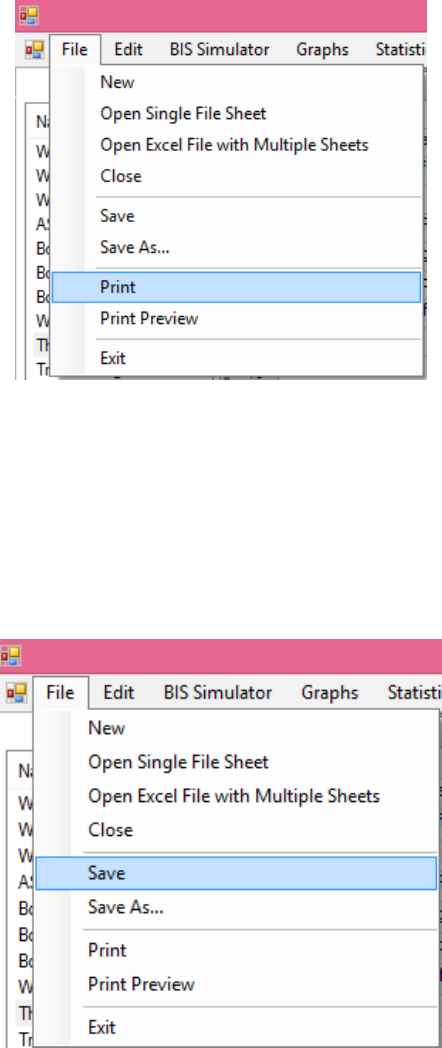
251
2. Click File ► Print or File ► Print Preview if you wish to see the preview before printing.
17.5 Saving Output Screens as Excel Files
ProUCL 5.0/ProUCL 5.1 saves output files and data files as Excel files with .xls or .xlsx extensions.
1. Click on the output you want to save in the Navigation Panel List.
2. Click File ► Save or File► Save As
3. Enter the desired file name you want to use, and click Save, and save the file in the desired folder
using your browser as shown below.
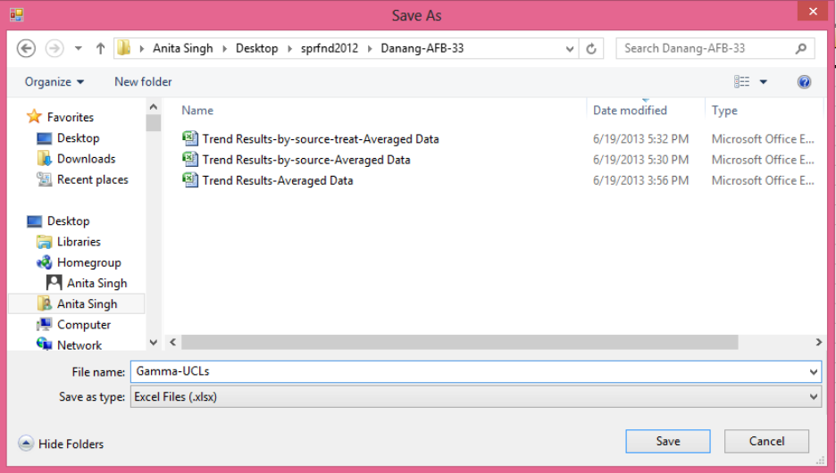
252

253
Chapter 18
Summary and Recommendations to Compute a 95% UCL for Full
Uncensored and Left-Censored Data Sets with NDs
This chapter briefly summarizes recommendations and the process to compute upper confidence limits of
the population mean based upon data sets with and without ND observations. The recommendations are
made based upon the simulation studies summarized in Singh, Singh, and Engelhardt (1997, 1999);
Singh, Singh, and Iaci (2002); Singh and Singh (2003); and Singh, Maichle, and Lee (2006). Some details
can be found in Chapters 2 and 4 of the associated ProUCL 5.1 Technical Guide. Depending upon the
data size, data distribution (e.g., normal, gamma, lognormal, and nonparametric), and data skewness,
ProUCL suggests using one or more 95% UCL to estimate the population mean. The project team
collectively should determine which of the suggested UCLs will be most appropriate for their project. If
needed, the user may want to consult a statistician for additional insight.
18.1 Computing UCL95s of the Mean Based Upon Uncensored Full Data Sets
Formal GOF tests and GOF Q-Q plots are used first to determine the data distribution so that
appropriate parametric or nonparametric UCL95s can be computed.
For a normally or approximately normally distributed data set, the user is advised to use Student’s
t-distribution-based UCL of the mean. Student’s t UCL or modified-t-statistic based UCL can be
used to estimate the EPC when the data set is symmetric (e.g., skewness =
3
ˆ
k
is smaller than 0.2-
0.3) or mildly skewed; that is, when σ or
σ
ˆ
is less than 0.5. In practice, for mildly skewed data
sets (with sd of logged data <0.5), all parametric UCLs computation methods available in
ProUCL tend to yield comparable results.
For gamma or approximately gamma distributed data sets, the user is advised to: 1) use the
approximate gamma UCL when k>1 and n ≥50; 2) use the adjusted gamma UCL when k>1 and
n<50; 3) use the bootstrap-t method or Hall’s bootstrap method when k ≤ 1 and the sample size, n
< 15-20; 4) use approximate gamma UCL for k ≤ 1 and sample size, n ≥ 50; and 5) use the
adjusted gamma UCL (if available) for k ≤ 1 and sample size, 50> n ≥ 15. If the adjusted gamma
UCL is not available (e.g., when an unusual CC level such as 0.935 is selected), then use the
approximate gamma UCL as an estimate of the EPC. When the bootstrap-t method or Hall’s
bootstrap method yields an erratic inflated UCL (e.g., when outliers are present) result, the UCL
may be computed using the adjusted gamma UCL (if available) or the approximate gamma UCL.
For lognormally distributed data sets, ProUCL recommends a UCL computation method based
upon the sample size, n, and standard deviation of the log-transformed data,
σ
ˆ
. These
suggestions are summarized in Table 2-10 of the ProUCL 5.1 Technical Guide.
For nonparametric data sets, which are not normally, lognormally, or gamma distributed, a
nonparametric UCL is used to estimate the EPC. Methods used to estimate EPC terms based
upon nonparametric data sets are summarized in Table 2-11 of the ProUCL 5.1 Technical Guide.
For example for mildly skewed nonparametric data sets of smaller sizes (e.g., <30), one may use
a modified-t UCL or BCA bootstrap UCL; and for larger samples one may use a CLT-UCL,
254
adjusted-CLT UCL, or a BCA bootstrap UCL. These nonparametric UCLs computation methods
do not provide desired coverage to the mean for moderately skewed to highly skewed data sets.
For moderately skewed to highly skewed nonparametric data sets, the use of a Chebyshev (Mean,
Sd) UCL is suggested. It is noted that for extremely skewed data sets (e.g., with
σ
ˆ
exceeding
3.0), even a Chebyshev inequality-based 99% UCL of the mean fails to provide the desired
coverage (e.g., 0.95) of the population mean.
For highly skewed data sets with
σ
ˆ
exceeding 3.0, 3.5, pre-processing the data is suggested. It is
very likely that the data consist of outliers and/or come from multiple populations. The
population partitioning methods may be used to identify mixture populations present in the data
set. For defensible conclusions, the decision statistics such as EPC terms may be computed
separately for each of the identified sub-population present in the mixture data set.
18.2 Computing UCLs Based Upon Left-Censored Data Sets with Nondetects
The parametric maximum likelihood estimation (MLE) methods (e.g., Cohen 1991) and expectation
maximization (EM) method (Gleit 1985) assume normality or lognormality of data sets and tend to work
only when the data set has NDs with only one detection limit. These days, due to modern analytical tools
and equipment, an environmental data sets consists of NDs with multiple detection limits. Since it is not
easy to verify (perform goodness-of-fit) the distribution of a left-censored data set consisting of detects
and NDs with multiple detection limits, some poor performing estimation methods including the
parametric MLE and EM methods and the winsorization method are not retained in ProUCL 5.0/ProUCL
5.1. In ProUCL, emphasis is given to the use of nonparametric UCL computation methods and hybrid
parametric methods based upon KM estimates which account for data skewness in the computation of
UCL95. Avoid the use of transformations (to achieve symmetry) while computing upper limits based
upon left-censored data sets. It is not easy to correctly interpret the statistics computed in the transformed
scale. Moreover, the results and statistics computed in the original scale do not suffer from transformation
bias. Like full uncensored data sets, when the standard deviation of the log-transformed data becomes
>1.0, avoid the use of a lognormal model even when the data appear to be lognormally distributed. Its
use often results in unrealistic statistics of no practical merit (Singh, Singh, and Engelhard 1997; Singh,
Singh, and Iaci 2002). It is also recommended to identify potential outliers representing observations
coming from population(s) different from the main dominant population and investigate them separately.
Decisions about the disposition of outliers should be made by all interested members of the project team.
It is recommended to avoid the use of the DL/2 (t) UCL method, as the DL/2 UCL does not
provide the desired coverage (for any distribution and sample size) for the population mean,
even for censoring levels as low as 10%, 15%. This is contrary to the conjecture and assertion
(e.g., EPA 2006a) made that the DL/2 method can be used for lower (e.g., ≤ 20%) censoring
levels. The coverage provided by the DL/2 (t) method deteriorates fast as the censoring
intensity increases. The DL/2 (t) method is not recommended by the authors or developers of
this text and ProUCL software.
The use of the KM estimation method is a preferred method as it can handle multiple
detection limits. Therefore, the use of KM estimates is suggested to compute the decision
statistics based upon methods which adjust for data skewness. Depending upon the data set
size, distribution of the detected data, and data skewness, the various nonparametric and
hybrid KM UCL95 methods including KM (BCA), bootstrap-t KM UCL, Chebyshev KM
255
UCL, Gamma-KM UCL based upon the KM estimates provide good coverages for the
population mean. All of these methods are available in ProUCL 5.1.

256
REFERENCES
Aitchison, J. and Brown, J.A.C. 1969. The Lognormal Distribution, Cambridge: Cambridge University
Press.
Anderson, T.W. and Darling, D. A. 1954. Test of goodness-of-fit. Journal of American Statistical
Association, Vol. 49, 765-769.
Bain, L.J., and Engelhardt, M. 1991. Statistical Analysis of Reliability and Life Testing Models, Theory
and Methods. 2
nd
Edition. Dekker, New York.
Bain, L.J. and Engelhardt, M. 1992. Introduction to probability and Mathematical Statistics. Second
Edition. Duxbury Press, California.
Barber, S. and Jennison, C. 1999. Symmetric Tests and Confidence Intervals for Survival Probabilities
and Quantiles of Censored Survival Data. University of Bath, Bath, BA2 7AY, UK.
Barnett, V. 1976. Convenient Probability Plotting Positions for the Normal Distribution. Appl. Statist.,
25, No. 1, pp. 47-50, 1976.
Barnett, V. and Lewis T. 1994. Outliers in Statistical Data. Third edition. John Wiley & Sons Ltd. UK.
Bechtel Jacobs Company, LLC. 2000. Improved Methods for Calculating Concentrations used in
Exposure Assessment. Prepared for DOE. Report # BJC/OR-416.
Best, D.J. and Roberts, D.E. 1975. The Percentage Points of the Chi-square Distribution. Applied
Statistics, 24: 385-388.
Best, D.J. 1983. A note on gamma variate generators with shape parameters less than unity. Computing,
30(2):185-188, 1983.
Blackwood, L. G. 1991. Assurance Levels of Standard Sample Size Formulas, Environmental Science and
Technology, Vol. 25, No. 8, pp. 1366-1367.
Blom, G. 1958. Statistical Estimates and Transformed Beta Variables. John Wiley and Sons, New York.
Bowman, K. O. and Shenton, L.R. 1988. Properties of Estimators for the Gamma Distribution, Volume
89. Marcel Dekker, Inc., New York.
Bradu, D. and Mundlak, Y. 1970. Estimation in Lognormal Linear Models. Journal of the American
Statistical Association, 65, 198-211.
Chen, L. 1995. Testing the Mean of Skewed Distributions. Journal of the American Statistical
Association, 90, 767-772.
Choi, S. C. and Wette, R. 1969. Maximum Likelihood Estimation of the Parameters of the Gamma
Distribution and Their Bias. Technometrics, Vol. 11, 683-690.

257
Cochran, W. 1977. Sampling Techniques, New York: John Wiley.
Cohen, A. C., Jr. 1950. Estimating the Mean and Variance of Normal Populations from Singly Truncated
and Double Truncated Samples. Ann. Math. Statist., Vol. 21, pp. 557-569.
Cohen, A. C., Jr. 1959. Simplified Estimators for the Normal Distribution When Samples Are Singly
Censored or Truncated. Technometrics, Vol. 1, No. 3, pp. 217-237.
Cohen, A. C., Jr. 1991. Truncated and Censored Samples. 119, Marcel Dekker Inc. New York, NY 1991.
Conover W.J.. 1999. Practical Nonparametric Statistics, 3rd Edition, John Wiley & Sons, New York.
D’Agostino, R.B. and Stephens, M.A. 1986. Goodness-of-Fit Techniques. Marcel Dekker, Inc.
Daniel, Wayne W. 1995. Biostatistics. 6th Edition. John Wiley & Sons, New York.
David, H.A. and Nagaraja, H.N. 2003. Order Statistics. Third Edition. John Wiley.
Department of Navy. 2002a. Guidance for Environmental Background Analysis. Volume 1 Soil. Naval
Facilities Engineering Command. April 2002.
Department of Navy. 2002b. Guidance for Environmental Background Analysis. Volume 2 Sediment.
Naval Facilities Engineering Command. May 2002.
Dixon, W.J. 1953. Processing Data for Outliers. Biometrics 9: 74-89.
Draper, N.R. and Smith, H. 1998. Applied Regression Analysis (3rd Edition). New York: John Wiley &
Sons.
Dudewicz, E.D. and Misra, S.N. 1988. Modern Mathematical Statistics. John Wiley, New York.
Efron, B. 1981. Censored Data and Bootstrap. Journal of American Statistical Association, Vol. 76, pp.
312-319.
Efron, B. 1982. The Jackknife, the Bootstrap, and Other Resampling Plans, Philadelphia: SIAM.
Efron, B. and Tibshirani, R.J. 1993. An Introduction to the Bootstrap. Chapman & Hall, New York.
El-Shaarawi, A.H. 1989. Inferences about the Mean from Censored Water Quality Data. Water Resources
Research, 25, pp. 685-690.
Fisher, R. A. 1936. The use of multiple measurements in taxonomic problems. Annals of Eugenics 7 (2):
179–188.
Fleischhauer, H. and Korte, N. 1990. Formation of Cleanup Standards Trace Elements with Probability
Plot. Environmental Management, Vol. 14, No. 1. 95-105.
Gehan, E.A. 1965. A Generalized Wilcoxon Test for Comparing Arbitrarily Singly-Censored Sample.
Biometrika 52, 203-223.

258
Gerlach, R. W., and J. M. Nocerino. 2003. Guidance for Obtaining Representative Laboratory Analytical
Subsamples from Particulate Laboratory Samples. EPA/600/R-03/027.
www.epa.gov/esd/tsc/images/particulate.pdf.
Gibbons. 1994. Statistical Methods for Groundwater Monitoring. John Wiley &Sons.
Gilbert, R.O. 1987. Statistical Methods for Environmental Pollution Monitoring. Van Nostrand Reinhold,
New York.
Gilliespie, B.W., Chen, Q., Reichert H., Franzblau A., Hedgeman E., Lepkowski J., Adriaens P., Demond
A., Luksemburg W., and Garabrant DH. 2010. Estimating population distributions when some data are
below a limit of detection by using a reverse Kaplan-Meier estimator. Epidemiology, Vol. 21, No. 4.
Gleit, A. 1985. Estimation for Small Normal Data Sets with Detection Limits. Environmental Science and
Technology, 19, pp. 1206-1213, 1985.
Grice, J.V., and Bain, L. J. 1980. Inferences Concerning the Mean of the Gamma Distribution. Journal of
the American Statistical Association. Vol. 75, Number 372, 929-933.
Gu, M.G., and Zhang, C.H. 1993. Asymptotic properties of self-consistent estimators based on doubly
censored data. Annals of Statistics. Vol. 21, 611-624.
Hahn, J. G. and Meeker, W.Q. 1991. Statistical Intervals. A Guide for Practitioners. John Wiley.
Hall, P. 1988. Theoretical comparison of bootstrap confidence intervals. Annals of Statistics, 16, 927-
953.
Hall, P. 1992. On the Removal of Skewness by Transformation. Journal of Royal Statistical Society, B 54,
221-228.
Hardin, J.W. and Gilbert, R.O. 1993. Comparing Statistical Tests for Detecting Soil Contamination
Greater Than Background. Pacific Northwest Laboratory, Battelle, Technical Report # DE 94-005498.
Hawkins, D. M., and Wixley, R. A. J. 1986. A Note on the Transformation of Chi-Squared Variables to
Normality. The American Statistician, 40, 296–298.
Hayes, A. F. 2005. Statistical Methods for Communication Science, Lawrence Erlbaum Associates,
Publishers.
Helsel, D.R. 2005. Nondetects and Data Analysis. Statistics for Censored Environmental Data. John
Wiley and Sons, NY.
Helsel, D.R. 2012. Statistics for Censored Environmental Data Using Minitab and R. Second Edition.
John Wiley and Sons, NY.
Helsel, D.R. 2102a. Practical Stats Webinar on ProUCL v4. The Unofficial User Guide; October 15,
2012.
Helsel, D.R. 2013. Nondetects and Data Analysis for Environmental Data, NADA in R
259
Helsel, D.R. and E. J. Gilroy. 2012. The Unofficial Users Guide to ProUCL4. Amazon, Kindle Edition.
Hinton, S.W. 1993.
Log-Normal Statistical Methodology Performance. ES&T Environmental Sci.
Technol., Vol. 27, No. 10, pp. 2247-2249.
Hoaglin, D.C., Mosteller, F., and Tukey, J.W. 1983. Understanding Robust and Exploratory Data
Analysis. John Wiley, New York.
Holgresson, M. and Jorner U. 1978. Decomposition of a Mixture into Normal Components: a Review.
Journal of Bio-Medicine. Vol. 9. 367-392.
Hollander M & Wolfe DA (1999). Nonparametric Statistical Methods (2nd Edition). New York: John
Wiley & Sons.
Hogg, R.V. and Craig, A. 1995. Introduction to Mathematical Statistics; 5
th
edition. Macmillan.
Huber, P.J. 1981, Robust Statistics, John Wiley and Sons, NY.
Hyndman, R. J. and Fan, Y. 1996. Sample quantiles in statistical packages, American Statistician, 50,
361–365.
Interstate Technology Regulatory Council (ITRC). 2012. Incremental Sampling Methodology. Technical
and Regulatory Guidance, 2012.
Interstate Technology Regulatory Council (ITRC). 2013 Groundwater Statistics and Monitoring
Compliance. Technical and Regulatory Guidance, December 2013.
Interstate Technology Regulatory Council (ITRC). 2015. Decision Making at Contaminated Sites.
Technical and Regulatory Guidance, January 2015.
Johnson, N.J. 1978. Modified-t-Tests and Confidence Intervals for Asymmetrical Populations. The
American Statistician, Vol. 73, 536-544.
Johnson, N.L., Kotz, S., and Balakrishnan, N. 1994. Continuous Univariate Distributions, Vol. 1. Second
Edition. John Wiley, New York.
Johnson, R.A. and D. Wichern. 2002. Applied Multivariate Statistical Analysis. 6
th
Edition. Prentice Hall.
Kaplan, E.L. and Meier, O. 1958. Nonparametric Estimation from Incomplete Observations. Journal of
the American Statistical Association, Vol. 53. 457-481.
Kleijnen, J.P.C., Kloppenburg, G.L.J., and Meeuwsen, F.L. 1986. Testing the Mean of an Asymmetric
Population: Johnson’s Modified-t Test Revisited. Commun. in Statist.-Simula., 15(3), 715-731.
Krishnamoorthy, K., Mathew, T., and Mukherjee, S. 2008. Normal distribution based methods for a
Gamma distribution: Prediction and Tolerance Interval and stress-strength reliability. Technometrics,
50, 69-78.

260
Kroese, D.P., Taimre, T., and Botev Z.I. 2011. Handbook of Monte Carlo Methods. John Wiley & Sons.
Kruskal, W. H., and Wallis, A. 1952. Use of ranks in one-criterion variance analysis. Journal of the
American Statistical Association, 47, 583-621.
Kupper, L. L. and Hafner, K. B. 1989, How Appropriate Are Popular Sample Size Formulas? The
American Statistician, Vol. 43, No. 2, pp. 101-105
Kunter, M. J., C. J. Nachtsheim, J. Neter, and Li W. 2004. Applied Linear Statistical Methods. Fifth
Edition. McGraw-Hill/Irwin.
Laga, J., and Likes, J. 1975, Sample Sizes for Distribution-Free Tolerance Intervals Statistical Papers.
Vol. 16, No. 1. 39-56
Land, C. E. 1971. Confidence Intervals for Linear Functions of the Normal Mean and Variance. Annals
of Mathematical Statistics, 42, pp. 1187-1205.
Land, C. E. 1975. Tables of Confidence Limits for Linear Functions of the Normal Mean and Variance. In
Selected Tables in Mathematical Statistics, Vol. III, American Mathematical Society, Providence, R.I.,
pp. 385-419.
Levene, Howard. 1960. Robust tests for equality of variances. In Olkin, Harold, et alia. Stanford
University Press. pp. 278–292.
Lilliefors, H.W. 1967. On the Kolmogorov-Smirnov Test for Normality with Mean and Variance
Unknown. Journal of the American Statistical Association, 62, 399-404.
Looney and Gulledge. 1985. Use of the Correlation Coefficient with Normal Probability Plots. The
American Statistician, 75-79.
Manly, B.F.J. 1997. Randomization, Bootstrap, and Monte Carlo Methods in Biology. Second Edition.
Chapman Hall, London.
Maronna, R.A., Martin, R.D., and Yohai, V.J. 2006, Robust Statistics: Theory and Methods, John Wiley
and Sons, Hoboken, NJ.
Marsaglia, G. and Tsang, W. 2000. A simple method for generating gamma variables. ACM Transactions
on Mathematical Software, 26(3):363-372.
Millard, S. P. and Deverel, S. J. 1988. Nonparametric statistical methods for comparing two sites based
on data sets with multiple nondetect limits. Water Resources Research, 24, pp. 2087-2098.
Millard, S.P. and Neerchal, M.K. 2002. Environmental Stats for S-PLUS. Second Edition. Springer.
Minitab version 16. 2012. Statistical Software.
261
Molin, P., and Abdi H. 1998. New Tables and numerical approximations for the Kolmogorov-
Smirnov/Lilliefors/ Van Soest’s test of normality. In Encyclopedia of Measurement and Statistics, Neil
Salkind (Editor, 2007). Sage Publication Inc. Thousand Oaks (CA).
Natrella, M.G. 1963. Experimental Statistics. National Bureau of Standards, Hand Book No. 91, U.S.
Government Printing Office, Washington, DC.
Noether, G.E. 1987 Sample Size Determination for some Common Nonparametric Tests, Journal
American Statistical Assoc., 82, 645-647
Perrson, T., and Rootzen, H. 1977. Simple and Highly Efficient Estimators for A Type I Censored Normal
Sample. Biometrika, 64, pp. 123-128.
Press, W.H., Flannery, B.P., Teukolsky, S.A., and Vetterling, W.T. 1990. Numerical Recipes in C, The
Art of Scientific Computing. Cambridge University Press. Cambridge, MA.
R Core Team, 2012. R: A language and environment for statistical computing. R Foundation for
Statistical Computing. Vienna, Austria. ISBN 3-900051-07-0, URL http://www.R-project.org/.
Rosner, B. 1975. On the detection of many outliers. Technometrics, 17, 221-227.
Rosner, B. 1983. Percentage points for a generalized ESD many-outlier procedure. Technometrics, 25,
165-172.
Rousseeuw, P.J. and Leroy, A.M. 1987. Robust Regression and Outlier Detection. John Wiley.
Royston, P. 1982. An extension of Shapiro and Wilk's W test for normality to large samples. Applied
Statistics, 31, 115–124.
Royston, P. 1982a. Algorithm AS 181: The W test for Normality. Applied Statistics, 31, 176–180.
Shacklette, H.T, and Boerngen, J.G. 1984. Element Concentrations in Soils and Other Surficial Materials
in the Conterminous United States, U.S. Geological Survey Professional Paper 1270.
Scheffe, H., and Tukey, J.W. 1944. A formula for Sample Sizes for Population Tolerance Limits. The
Annals of Mathematical Statistics. Vol 15, 217.
Schulz, T. W. and Griffin, S. 1999. Estimating Risk Assessment Exposure Point Concentrations when
Data are Not Normal or Lognormal. Risk Analysis, Vol. 19, No. 4.
Scheffe, H., and Tukey, J.W. 1944. A formula for Sample Sizes for Population Tolerance Limits. The
Annals of Mathematical Statistics. Vol 15, 217.
Schneider, B.E. and Clickner, R.P. 1976. On the Distribution of the Kolmogorov-Smirnov Statistic for the
Gamma Distribution with Unknown Parameters. Mimeo Series Number 36, Department of Statistics,
School of Business Administration, Temple University, Philadelphia, PA.
Schneider, B. E. 1978. Kolmogorov-Smirnov Test Statistic for the Gamma Distribution with Unknown
Parameters, Dissertation, Department of Statistics, Temple University, Philadelphia, PA.

262
Schneider, H. 1986. Truncated and Censored Samples from Normal Populations. Vol. 70, Marcel Dekker
Inc., New York, 1986.
She, N. 1997. Analyzing Censored Water Quality Data Using a Nonparametric Approach. Journal of the
American Water Resources Association 33, pp. 615-624.
Shea, B. 1988. Algorithm AS 239: Chi-square and Incomplete Gamma Integrals. Applied Statistics, 37:
466-473.
Shumway, A.H., Azari, A.S., Johnson, P. 1989. Estimating Mean Concentrations Under Transformation
for Environmental Data with Detection Limits. Technometrics, Vol. 31, No. 3, pp. 347-356.
Shumway, R.H., R.S. Azari, and M. Kayhanian. 2002. Statistical Approaches to Estimating Mean Water
Quality Concentrations with Detection Limits. Environmental Science and Technology, Vol. 36, pp.
3345-3353.
Sinclair, A.J. 1976. Applications of Probability Graphs in Mineral Exploration. Association of
Exploration Geochemists, Rexdale Ontario, p 95.
Singh, A. 1993. Omnibus Robust Procedures for Assessment of Multivariate Normality and Detection of
Multivariate Outliers. In Multivariate Environmental Statistics, Patil G.P. and Rao, C.R., Editors, pp.
445-488. Elsevier Science Publishers.
Singh, A. 2004. Computation of an Upper Confidence Limit (UCL) of the Unknown Population Mean
Using ProUCL Version 3.0. Part I. Download from: www.epa.gov/nerlesd1/tsc/issue.htm
Singh, A., Maichle, R., and Lee, S. 2006. On the Computation of a 95% Upper Confidence Limit of the
Unknown Population Mean Based Upon Data Sets with Below Detection Limit Observations.
EPA/600/R-06/022, March 2006. http://www.epa.gov/osp/hstl/tsc/softwaredocs.htm
Singh, A. and Nocerino, J.M. 1995. Robust Procedures for the Identification of Multiple Outliers.
Handbook of Environmental Chemistry, Statistical Methods, Vol. 2.G, pp. 229-277. Springer Verlag,
Germany.
Singh, A. and Nocerino, J.M. 1997. Robust Intervals for Some Environmental Applications." The Journal
of Chemometrics and Intelligent Laboratory Systems, Vol 37, 55-69.
Singh, A. and Nocerino, J.M. 2002. Robust Estimation of the Mean and Variance Using Environmental
Data Sets with Below Detection Limit Observations, Vol. 60, pp 69-86.
Singh, A.K. and Ananda. M. 2002. Rank kriging for characterization of mercury contamination at the
East Fork Poplar Creek, Oak Ridge, Tennessee. Environmetrics, Vol. 13, pp. 679-691.
Singh, A. and Singh, A.K. 2007. ProUCL Version 4 Technical Guide (Draft). Publication EPA/600/R-
07/041. January, 2007. http://www.epa.gov/osp/hstl/tsc/softwaredocs.htm
Singh, A. and Singh, A.K. 2009. ProUCL Version 4.00.04 Technical Guide (Draft). Publication
EPA/600/R-07/041. February, 2009. http://www.epa.gov/osp/hstl/tsc/softwaredocs.htm
263
Singh, A.K., Singh, A., and Engelhardt, M. 1997. The Lognormal Distribution in Environmental
Applications. Technology Support Center Issue Paper, 182CMB97. EPA/600/R-97/006, December 1997.
Singh, A., Singh A.K., and Engelhardt, M. 1999, Some Practical Aspects of sample Size and Power
Computations for Estimating the Mean of Positively Skewed Distributions in Environmental Applications.
Office of Research and Development. EPA/006/s-99/006. November 1999.
http://www.epa.gov/esd/tsc/images/325cmb99rpt.pdf
Singh, A., Singh, A.K., and Flatman, G. 1994. Estimation of Background Levels of Contaminants. Math
Geology, Vol. 26, No, 3, 361-388.
Singh, A., Singh, A.K., and Iaci, R.J. 2002. Estimation of the Exposure Point Concentration Term Using
a Gamma Distribution, EPA/600/R-02/084, October 2002.
Stephens, M. A. 1970. Use of Kolmogorov-Smirnov, Cramer-von Mises and Related Statistics Without
Extensive Tables. Journal of Royal Statistical Society, B 32, 115-122.
Sutton, C.D. 1993. Computer-Intensive Methods for Tests About the Mean of an Asymmetrical
Distribution. Journal of American Statistical Society, Vol. 88, No. 423, 802-810.
Tarone, R. and Ware, J. 1978. On Distribution-free Tests for Equality of Survival Distributions.
Biometrika, 64, 156-160.
Thom, H.C.S. 1968. Direct and Inverse Tables of the Gamma Distribution. Silver Spring, MD;
Environmental Data Service.
U.S. Environmental Protection Agency (EPA). 1989a. Methods for Evaluating the Attainment of Cleanup
Standards, Vol. 1, Soils and Solid Media. Publication EPA 230/2-89/042.
U.S. Environmental Protection Agency (EPA). 1989b. Statistical Analysis of Ground-water Monitoring
Data at RCRA Facilities. Interim Final Guidance. Washington, DC: Office of Solid Waste. April 1989.
U.S. Environmental Protection Agency (EPA). 1991. A Guide: Methods for Evaluating the Attainment of
Cleanup Standards for Soils and Solid Media. Publication EPA/540/R95/128.
U.S. Environmental Protection Agency (EPA). 1992a. Supplemental Guidance to RAGS: Calculating the
Concentration Term. Publication EPA 9285.7-081, May 1992.
U.S. Environmental Protection Agency (EPA). 1992b. Statistical Analysis of Ground-water Monitoring
Data at RCRA Facilities. Addendum to Interim Final Guidance. Washington DC: Office of Solid Waste.
July 1992.
U.S. Environmental Protection Agency (EPA). 1994. Statistical Methods for Evaluating the Attainment of
Cleanup Standards, EPA 230-R-94-004, Washington, DC.
U.S. Environmental Protection Agency (EPA). 1996. A Guide: Soil Screening Guidance: Technical
Background Document. Second Edition, Publication 9355.4-04FS.

264
U.S. Environmental Protection Agency (EPA). MARSSIM. 2000. U.S. Nuclear Regulatory Commission,
et al. Multi-Agency Radiation Survey and Site Investigation Manual (MARSSIM). Revision 1. EPA 402-
R-97-016. Available at http://www.epa.gov/radiation/marssim/ or from
http://bookstore.gpo.gov/index.html (GPO Stock Number for Revision 1 is 052-020-00814-1).
U.S. Environmental Protection Agency (EPA). 2002a. Calculating Upper Confidence Limits for Exposure
Point Concentrations at Hazardous Waste Sites. OSWER 9285.6-10. December 2002.
U.S. Environmental Protection Agency (EPA). 2002b. Guidance for Comparing Background and
Chemical Concentrations in Soil for CERCLA Sites. EPA 540-R-01-003-OSWER 9285.7-41. September
2002.
U.S. Environmental Protection Agency (EPA). 2002c. RCRA Waste Sampling, Draft Technical Guidance
– Planning, Implementation and Assessment. EPA 530-D-02-002, 2002.
U.S. Environmental Protection Agency (EPA). 2004. ProUCL Version 3.1, Statistical Software. National
Exposure Research Lab, EPA, Las Vegas Nevada, October 2004.
http://www.epa.gov/osp/hstl/tsc/softwaredocs.htm
U.S. Environmental Protection Agency (EPA). 2006a, Guidance on Systematic Planning Using the Data
Quality Objective Process, EPA QA/G-4, EPA/240/B-06/001. Office of Environmental Information,
Washington, DC. Download from: http://www.epa.gov/quality/qs-docs/g4-final.pdf
U.S. Environmental Protection Agency (EPA). 2006b. Data Quality Assessment: Statistical Methods for
Practitioners, EPA QA/G-9S. EPA/240/B-06/003. Office of Environmental Information, Washington,
DC. Download from: http://www.epa.gov/quality/qs-docs/g9s-final.pdf
U.S. Environmental Protection Agency (EPA). 2007. ProUCL Version 4.0 Technical Guide. EPA 600-R-
07-041, January 2007.
U.S. Environmental Protection Agency (EPA). 2009. Statistical Analysis of Groundwater Monitoring
Data at RCRA Facilities – Unified Guidance. EPA 530-R-09-007, 2009.
U.S. Environmental Protection Agency (EPA). 2009a. ProUCL Version 4.00.05 User Guide (Draft).
Statistical Software for Environmental Applications for Data Sets with and without nondetect
observations. National Exposure Research Lab, EPA, Las Vegas. EPA/600/R-07/038, February 2009.
Down load from: http://www.epa.gov/osp/hstl/tsc/softwaredocs.htm
U.S. Environmental Protection Agency (EPA). 2009b. ProUCL Version 4.00.05 Technical Guide (Draft).
Statistical Software for Environmental Applications for Data Sets with and without nondetect
observations. National Exposure Research Lab, EPA, Las Vegas. EPA/600/R-07/038, February 2009.
Down load from: http://www.epa.gov/osp/hstl/tsc/softwaredocs.htm
U.S. Environmental Protection Agency (EPA). 2009c. ProUCL4.00.05 Facts Sheet. Statistical Software
for Environmental Applications for Data Sets with and without nondetect observations. National
Exposure Research Lab, EPA, Las Vegas, Nevada, 2009.
http://www.epa.gov/osp/hstl/tsc/softwaredocs.htm

265
U.S. Environmental Protection Agency (EPA). 2009d. Scout 2008 – A Robust Statistical Package, Office
of Research and Development, February 2009.
http://archive.epa.gov/esd/archive-scout/web/html/
U.S. Environmental Protection Agency (EPA). 2010. Scout 2008 User Guide (Draft) EPA/600/R-08/038,
Office of Research and Development, April 2010.
http://archive.epa.gov/esd/archive-scout/web/html/
U.S. Environmental Protection Agency (EPA). 2010a. A Quick Guide to the Procedures in Scout (Draft),
Office of Research and Development, April 2010.
http://archive.epa.gov/esd/archive-scout/web/html/
U.S. Environmental Protection Agency (EPA). 2010b. ProUCL Version 4.00.05 User Guide (Draft).
EPA/600/R-07/041, May 2010. http://www.epa.gov/osp/hstl/tsc/software.htm
U.S. Environmental Protection Agency (EPA). 2010c. ProUCL Version 4.00.05 Technical Guide (Draft).
EPA/600/R-07/041, May, 2010. http://www.epa.gov/osp/hstl/tsc/software.htm
U.S. Environmental Protection Agency (EPA). 2010d. ProUCL 4.00.05, Statistical Software for
Environmental Applications for Data Sets with and without nondetect observations. National Exposure
Research Lab, EPA, Las Vegas Nevada, May 2010. http://www.epa.gov/osp/hstl/tsc/softwaredocs.htm
U.S. Environmental Protection Agency (EPA). 2011. ProUCL 4.1.00, Statistical Software for
Environmental Applications for Data Sets with and without nondetect observations. National Exposure
Research Lab, EPA, Las Vegas Nevada, June 2011. http://www.epa.gov/osp/hstl/tsc/softwaredocs.htm
U.S. Environmental Protection Agency (EPA). 2013a. ProUCL 5.0.00 Technical Guide (Draft)
EPA/600/R-07/041. September 2013. Office of Research and Development.
http://www.epa.gov/esd/tsc/TSC_form.htm
U.S. Environmental Protection Agency (EPA). 2013b. ProUCL 5.0.00 User Guide (Draft) EPA/600/R-
07/041. September 2013. Office of Research and Development.
http://www.epa.gov/esd/tsc/TSC_form.htm
U.S. Environmental Protection Agency (EPA). 2014. ProUCL 5.0.00 Statistical Software for
Environmental Applications for Datasets with and without Nondetect Observations, Office of Research
and Development, August 2014. http://www.epa.gov/esd/tsc/TSC_form.htm
Wald, A. 1943. An Extension of Wilks’ Method for Setting Tolerance Intervals. Annals of Mathematical
Statistics. Vol. 14, 44-55.
Whittaker, J. 1974. Generating Gamma and Beta Random Variables with Non-integral Shape
Parameters. Applied Statistics, 23, No. 2, 210-214.
Wilks, S.S. 1941. Determination of Sample Sizes for Setting Tolerance Limits. Annals of Mathematical
Statistics, Vol. 12, 91-96.
Wilks, S.S. 1963. Multivariate statistical outliers. Sankhya A, 25: 407-426.
266
Wilson, E.B., and Hilferty, M.M. 1931, “The Distribution of Chi-Squares,” Proceedings of the National
Academy of Sciences, 17, 684–688.
Wong, A. 1993. A Note on Inference for the Mean Parameter of the Gamma Distribution. Statistics
Probability Letters, Vol. 17, 61-66.

267

268
Office of Research
and Development (8101R)
Washington, DC 20460
Official Business
Penalty for Private Use
$300
EPA/600/R-07/038
Februaryl 2009
www.epa.gov
PRESORTED STANDARD
POSTAGE & FEES PAID
EPA
PERMIT No. G-35
Please make all necessary changes on the below label,
detach or copy, and return to the address in the upper
left-hand corner.
If you do not wish to receive these reports CHECK HERE
□
; detach, or copy this cover, and return to the address in the
upper left-hand corner.
Recycled/Recyclable
Printed with vegetable-based ink on
paper that contains a minimum of
50% post-consumer fiber content
processed chlorine free
v
